If you follow information security discussions on the internet, you might have heard that blurring an image is not a good way of redacting its contents. This is supposedly because blurring algorithms are reversible.
But then, it’s not wrong to scratch your head. Blurring amounts to averaging the underlying pixel values. If you average two numbers, there’s no way of knowing if you’ve started with 1 + 5 or 3 + 3. In both cases, the arithmetic mean is the same and the original information appears to be lost. So, is the advice wrong?
Well, yes and no! There are ways to achieve non-reversible blurring using deterministic algorithms. That said, in other cases, blur filters can preserve far more information than would appear to the naked eye — and do so in a pretty unexpected way. In today’s article, we’ll build a rudimentary blur algorithm and then pick it apart.
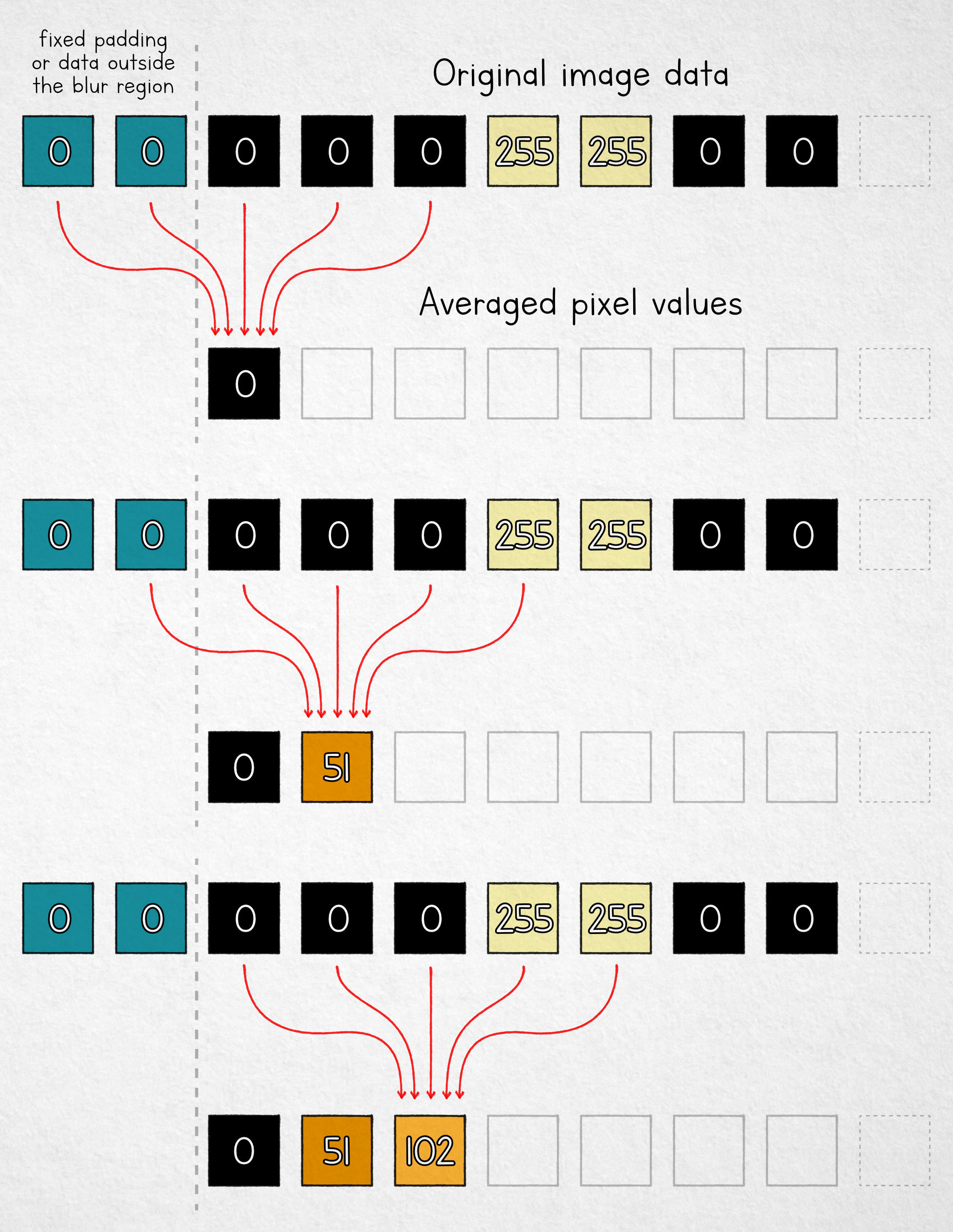
If blurring is the same as averaging, then the simplest algorithm we can choose is the moving mean. We take a fixed-size window and replace each pixel value with the arithmetic mean of n pixels in its neighborhood. For n = 5, the process is shown below:
[

Moving average as a simple blur algorithm.
Note that for the first two cells, we don’t have enough pixels in the input buffer. We can use fixed padding, “borrow” some available pixels from outside the selection area, or simply average fewer values near the boundary. Either way, the analysis doesn’t change much.
Let’s assume that we’ve completed the blurring process and no longer have the original pixel values. Can the underlying image be reconstructed? Yes, and it’s simpler than one might expect. We don’t need big words like “deconvolution”, “point spread function”, “kernel”, or any scary-looking math.
We start at the left boundary (x = 0). Recall that we calculated the first blurred pixel like by averaging the following pixels in the original image:
\(blur(0) = {img(-2) \ + \ img(-1) \ + \ img(0) \ +\ img(1)\ +\ img(2) \over 5}\)
Next, let’s have a look at the blurred pixel at x = 1. Its value is the average of:
\(blur(1) = {img(-1)\ +\ img(0)\ +\ img(1)\ +\ img(2)\ +\ img(3) \over 5}\)
We can easily turn these averages into sums by multiplying both sides by the number of averaged elements (5):
\(\begin{align} 5 \cdot blur(0) &= img(-2) + \underline{img(-1) + img(0) + img(1) + img(2)} \\ 5 \cdot blur(1) &= \underline{img(-1) + img(0) + img(1) + img(2)} + img(3) \end{align} \)
Note that the underlined terms repeat in both expressions; this means that if we subtract the expressions from each other, we end up with just:
\(5 \cdot blur(1) - 5 \cdot blur(0) = img(3) - img(-2) \)
The value of img(-2) is known to us: it’s one of the fixed padding pixels used by the algorithm. Let’s shorten it to c. We also know the values of blur(0) and blur(1): these are the blurred pixels that can be found in the output image. This means that we can rearrange the equation to recover the original input pixel corresponding to img(3):
\(img(3) = 5 \cdot (blur(1) - blur(0)) + c\)
We can also apply the same reasoning to the next pixel:
\(img(4) = 5 \cdot (blur(2) - blur(1)) + c\)
At this point, we seemingly hit a wall with our five-pixel average, but the knowledge of img(3) allows us to repeat the same analysis for the blur(5) / blur(6) pair a bit further down the line:
\(\begin{align} 5 \cdot blur(5) &= img(3) + \underline{img(4) + img(5) + img(6) + img(7)} \\ 5 \cdot blur(6) &= \underline{img(4) + img(5) + img(6) + img(7)} + img(8) \\ \\ img(8) &= 5 \cdot (blur(6) - blur(5)) + img(3) \end{align} \)
This nets us another original pixel value, img(8). From the earlier step, we also know the value of img(4), so we can find img(9) in a similar way. This process can continue to successively reconstruct additional pixels, although we end up with some gaps. For example, following the calculations outlined above, we still don’t know the value of img(0) or img(1).
These gaps can be resolved with a second pass that moves in the opposite direction in the image buffer. That said, instead of going down that path, we can also make the math a bit more orderly with a good-faith tweak to the averaging algorithm.
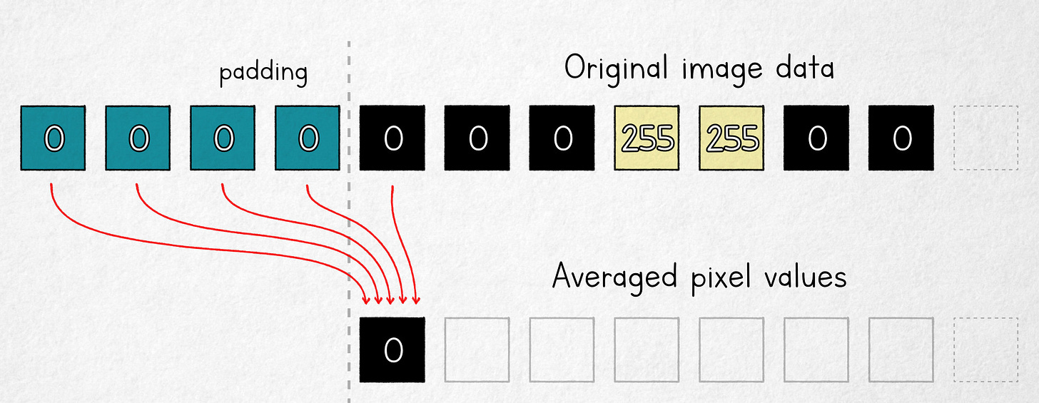
The modification that will make our life easier is to shift the averaging window so that one of its ends is aligned with where the computed value will be stored:
[
Moving average with a right-aligned window.
In this model, the first output value is an average of four fixed padding pixels (c) and one original image pixel; it follows that in the n = 5 scenario, the underlying pixel value can be computed as:
\(img(0) = 5 \cdot blur(0) - 4 \cdot c\)
If we know img(0), we now have all but one of the values that make up blur(1), so we can find img(1):
\(img(1) = 5 \cdot blur(1) - 3 \cdot c - img(0)\)
The process can be continued iteratively, reconstructing the entire image — this time, without any discontinuities and without the need for a second pass.
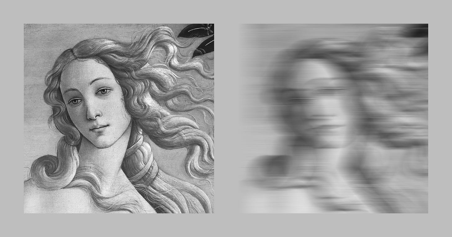
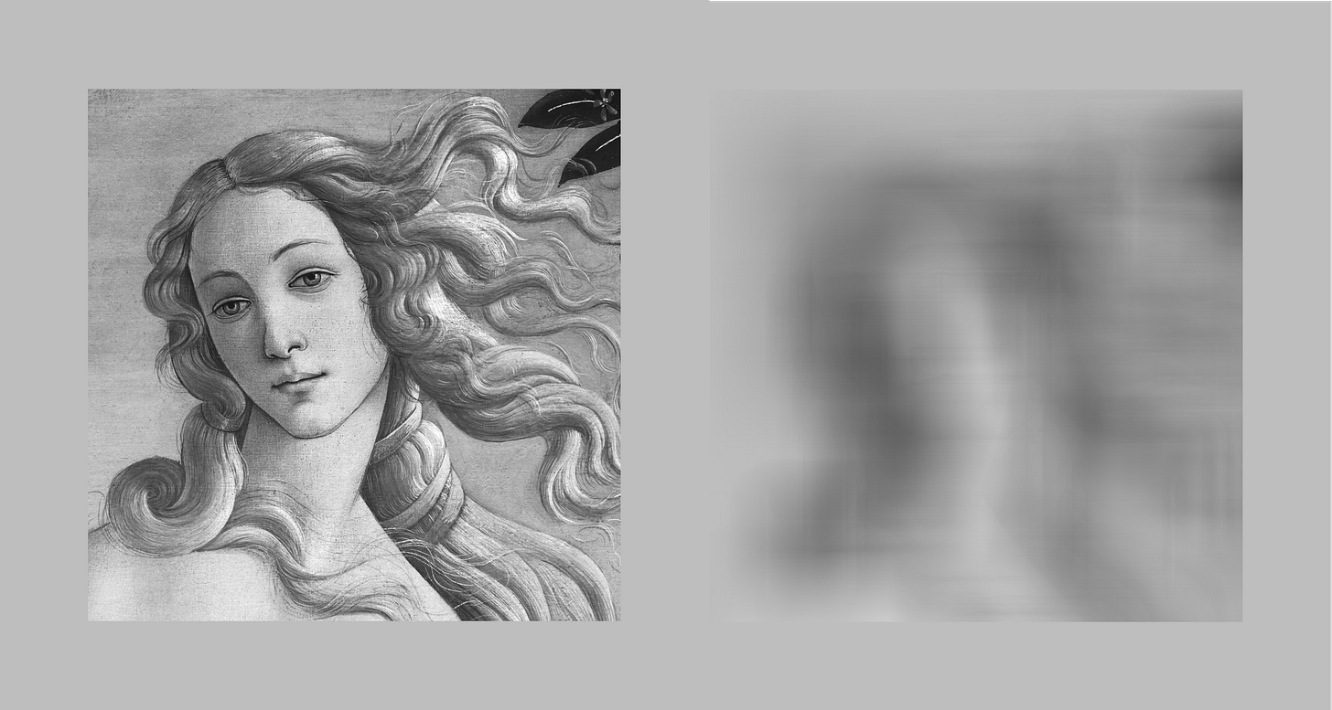
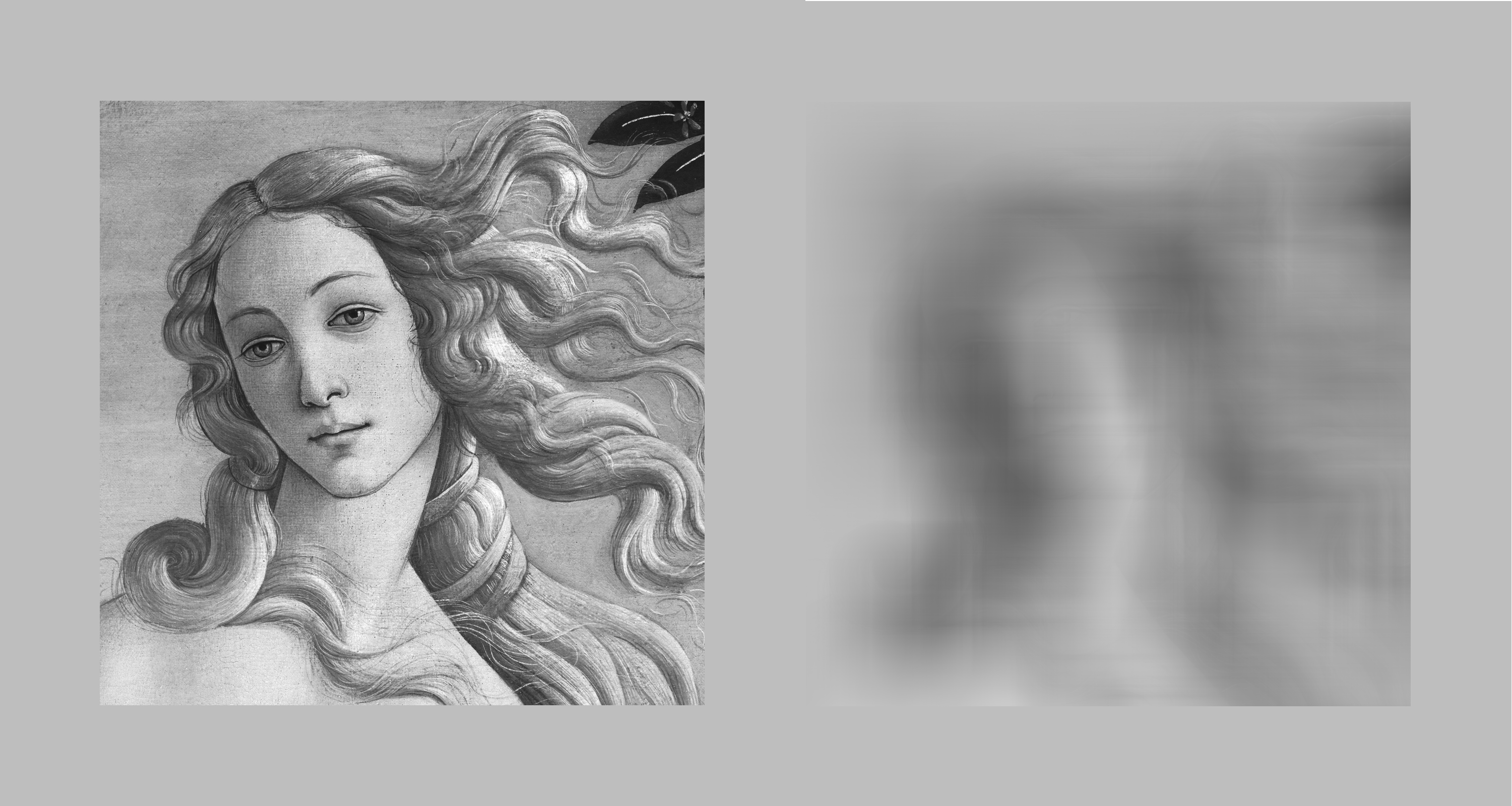
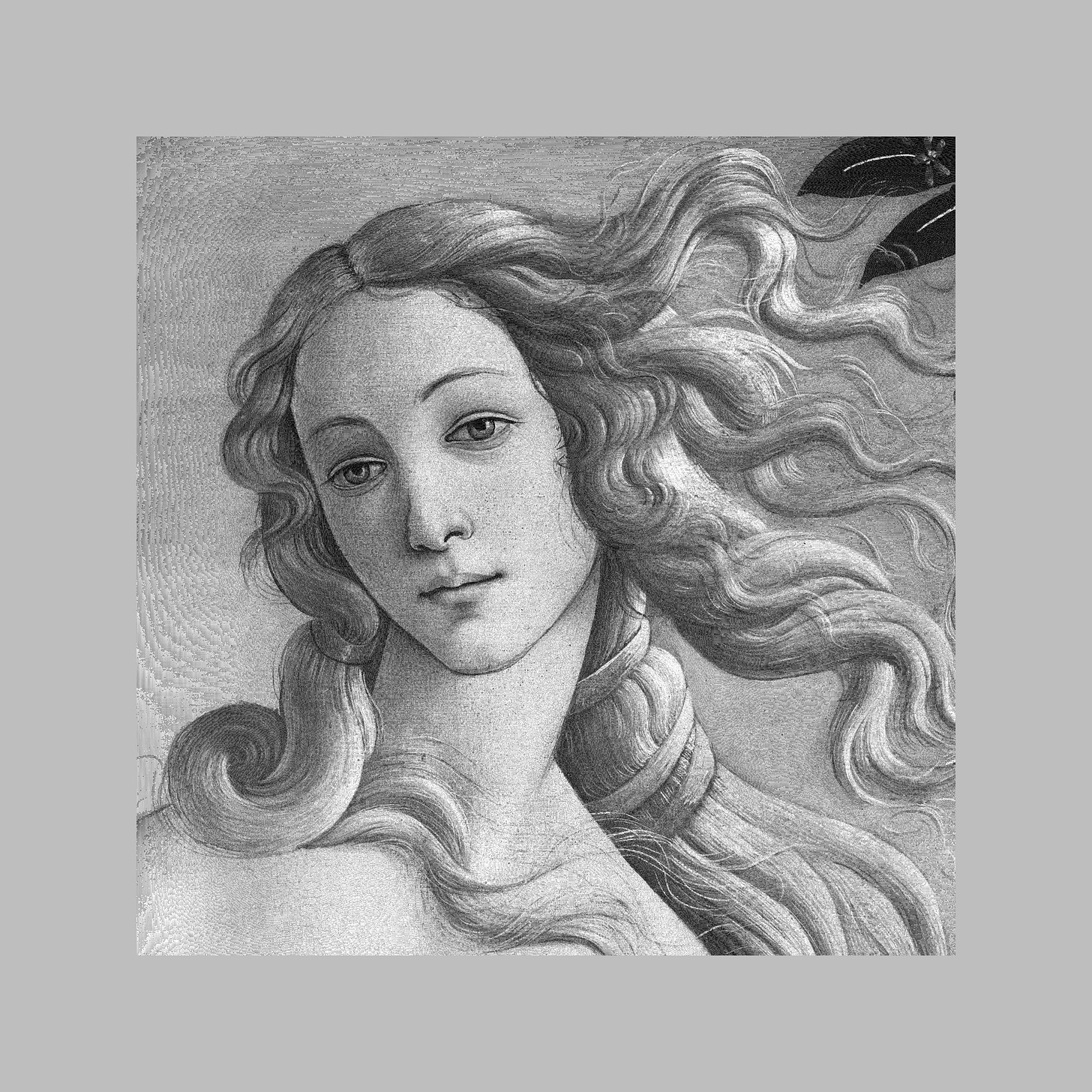
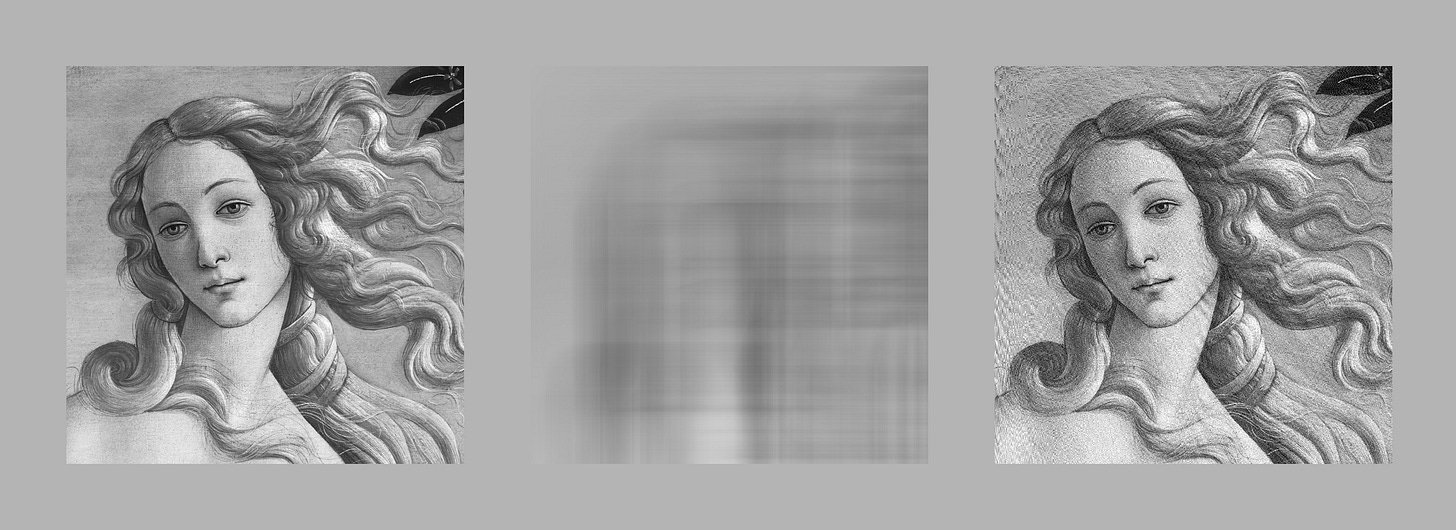
In the illustration below, the left panel shows a detail of The Birth of Venus by Sandro Botticelli; the right panel is the same image ran through the right-aligned moving average blur algorithm with a 151-pixel averaging window that moves only in the x direction:
[
Venus, x-axis moving average.
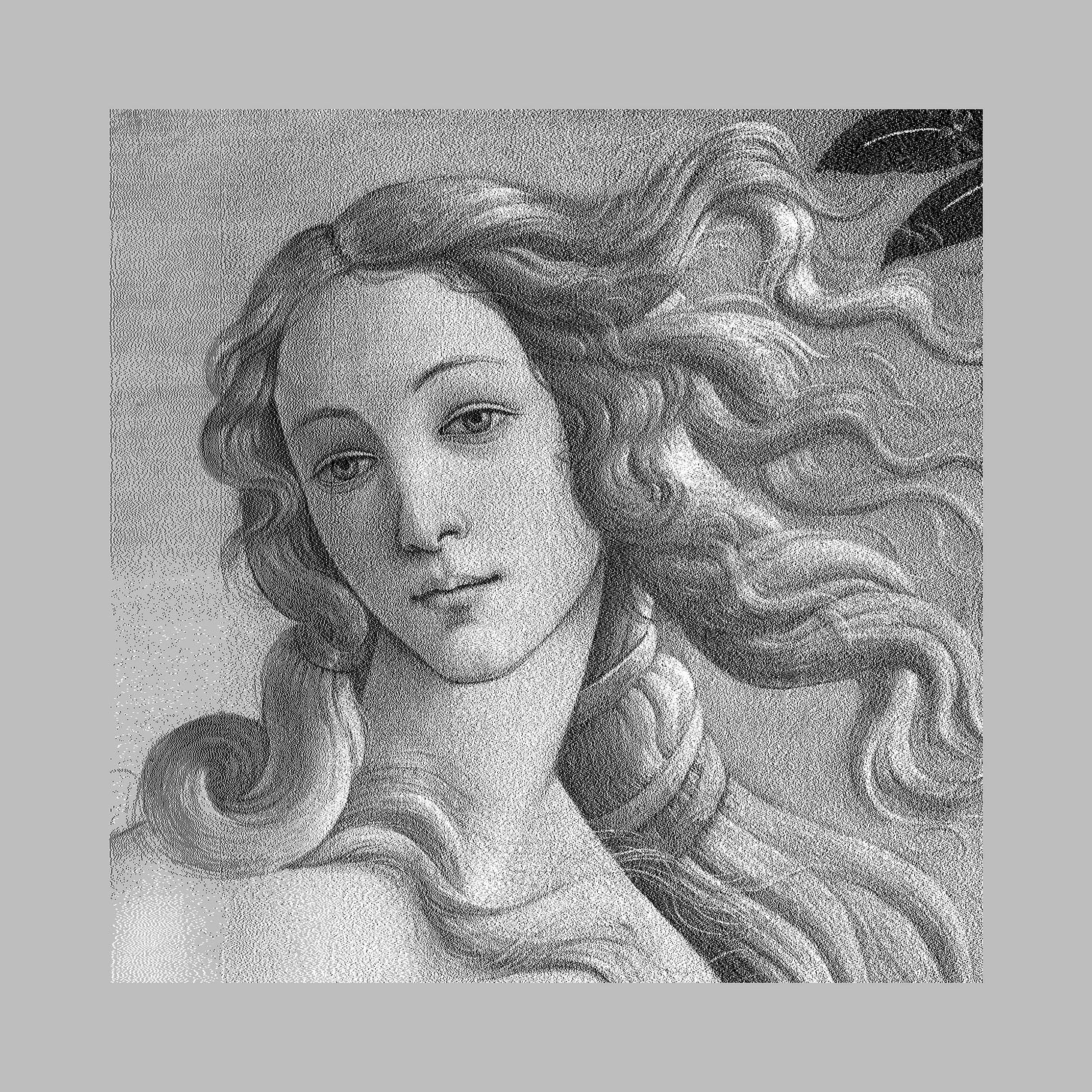
Now, let’s take the blurry image and attempt the reconstruction method outlined above — computer, ENHANCE!
[
The Rebirth of Venus.
This is rather impressive. The image is noisier than before as a consequence of 8-bit quantization of the averaged values in the intermediate blurred image. Nevertheless, even with a large averaging window, fine detail — including individual strands of hair — could be recovered and is easy to discern.
The problem with our blur algorithm is that it averages pixel values only in the x axis; this gives the appearance of motion blur or camera shake.
The approach we’ve developed can be extended to a 2D filter with a square-shaped or a cross-shaped averaging window. That said, a more expedient hack is to apply the existing 1D filter in the x axis and then follow with a complementary pass in the y axis. To undo the blur, we’d then perform two recovery passes in the inverse order.
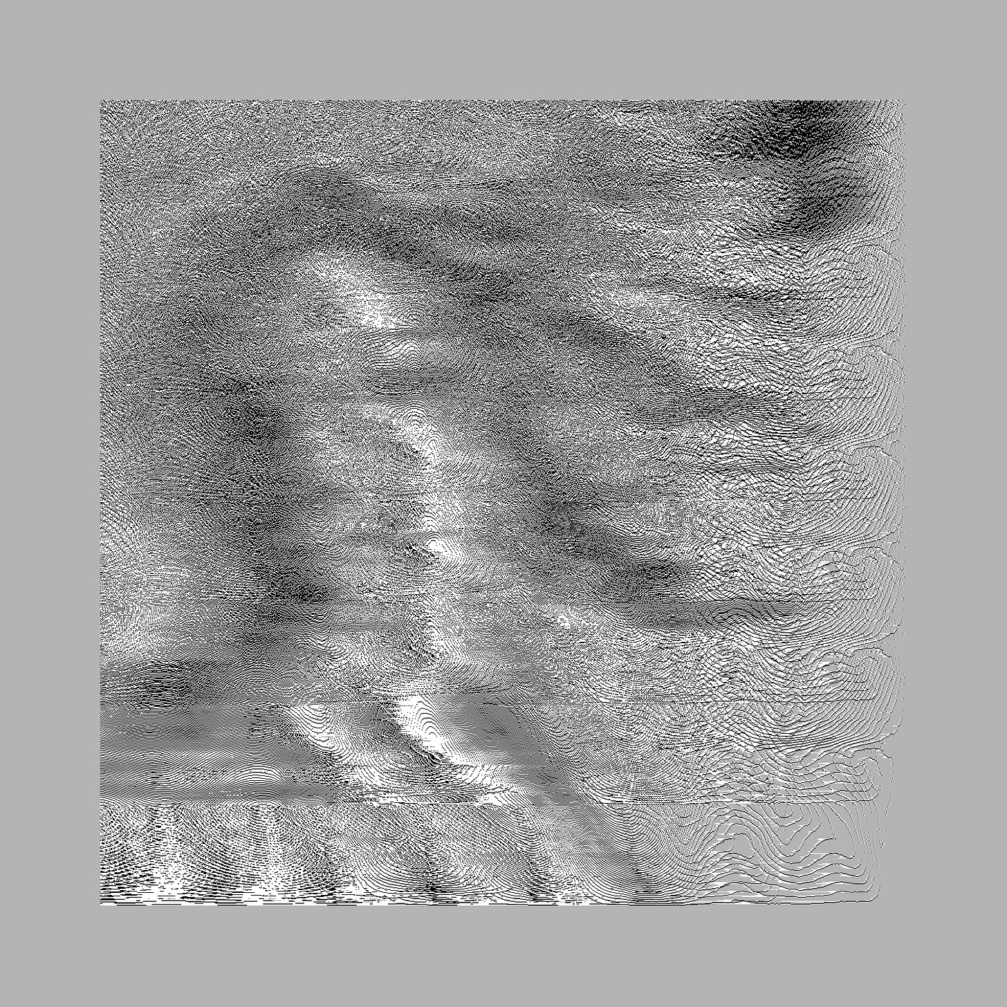
Unfortunately, whether we take the 1D + 1D or the true 2D route, we’ll discover that the combined amount of averaging per pixel causes the underlying values to be quantized so severely that the reconstructed image is overwhelmed by noise unless the blur window is relatively small:
[
Reconstruction from a 1D + 1D moving-average blur (x followed by y).
That said, if we wanted to develop an adversarial blur filter, we could fix the problem by weighting the original pixel a bit more heavily in the calculated mean. For the x-then-y variant, if the averaging window has a size W and the current-pixel bias factor is B, we can write the following formula:
\(blur(n) = {img(n - W) + \ldots + img(n - 1) + B \cdot img(n) \over W + B}\)
This filter still does what it’s supposed to do; here’s the output of an x-then-y blur for W = 200 and B = 30:
[
Venus, heavy X-Y blur.
Surely, there’s no coming back from tha— COMPUTER, ENHANCE!
[
Venus, recovered from a heavy blur.
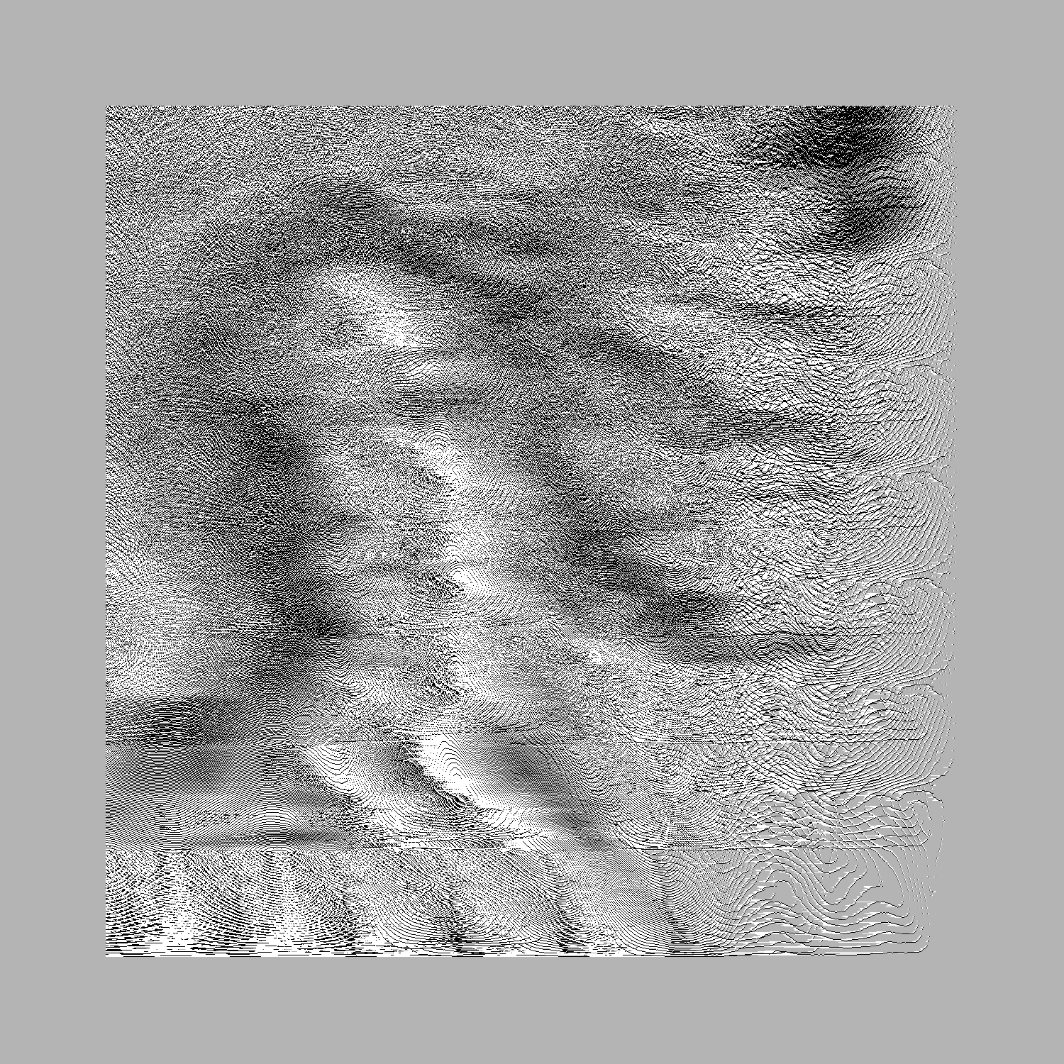
As a proof of concept for skeptics, we can also make an adversarial filter that operates in two dimensions simultaneously. The following is a reconstruction after a 2D filter with a simple cross-shaped window:
[
Reconstruction from a simultaneous 2D filter (W = 600×600, B = 10).
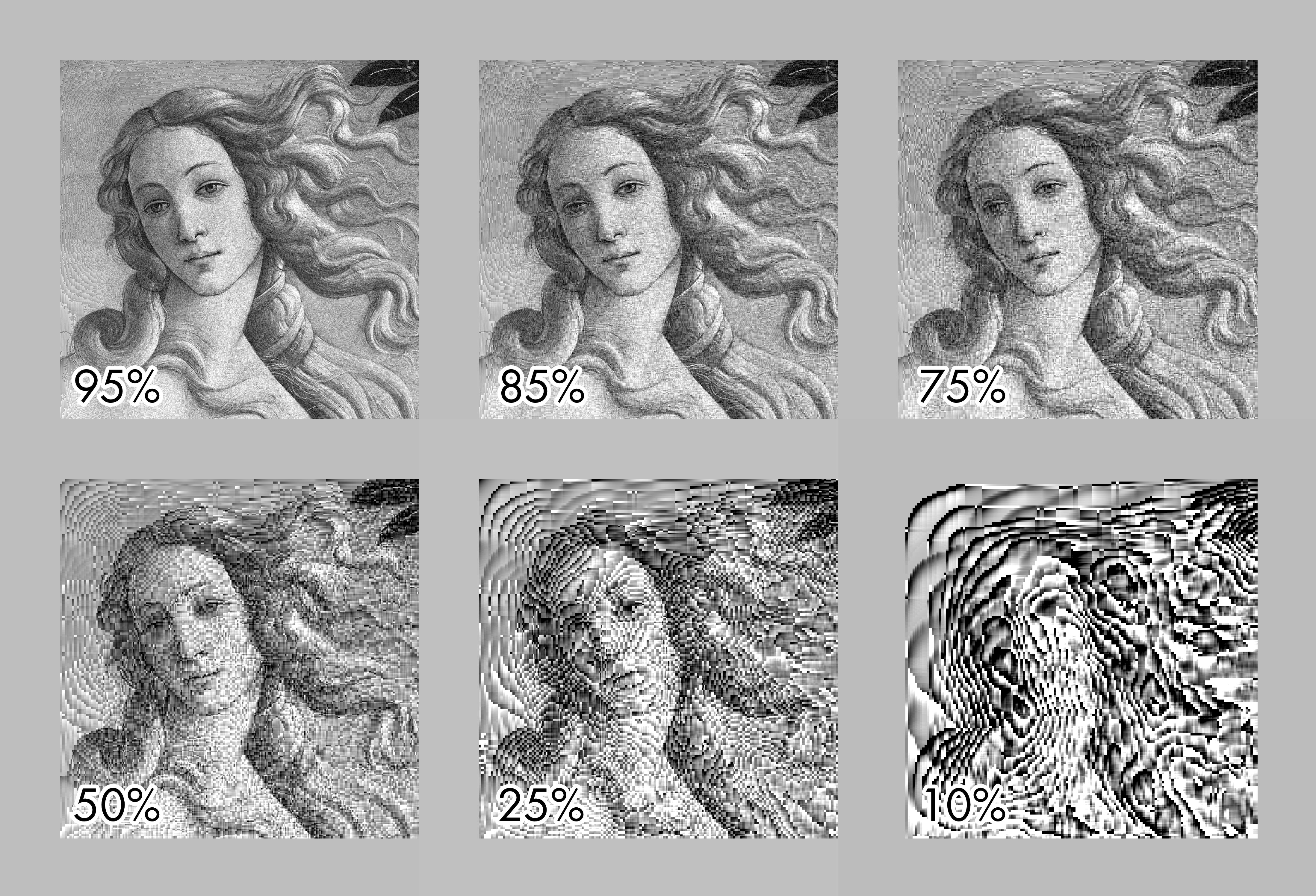
Remarkably, the information “hidden” in the blurred images survives being saved in a lossy image format. The top row shows images reconstituted from an intermediate image saved as a JPEG at 95%, 85%, and 75% quality settings:
[

Recovery from a JPEG file (1D + 1D filter, W = 200, B = 30).
The bottom row shows less reasonable quality settings of 50% and below; at that point, the reconstructed image begins to resemble abstract art.
For more weird algorithms, click here or here. Thematic catalog of posts on this site can be found on this page.
No posts