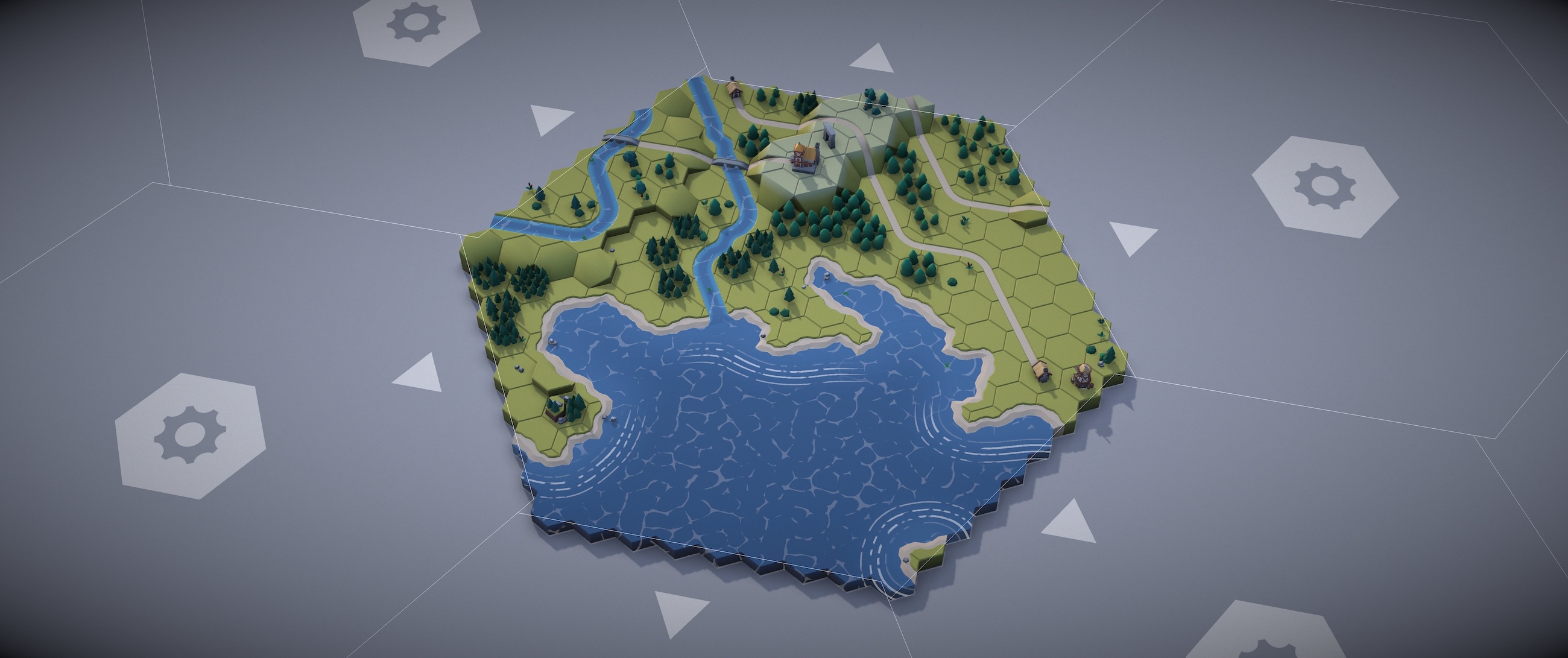
Procedural medieval islands from 4,100 hex tiles, built with WebGPU and a lot of backtracking.

Run the live demo · Source code on GitHub

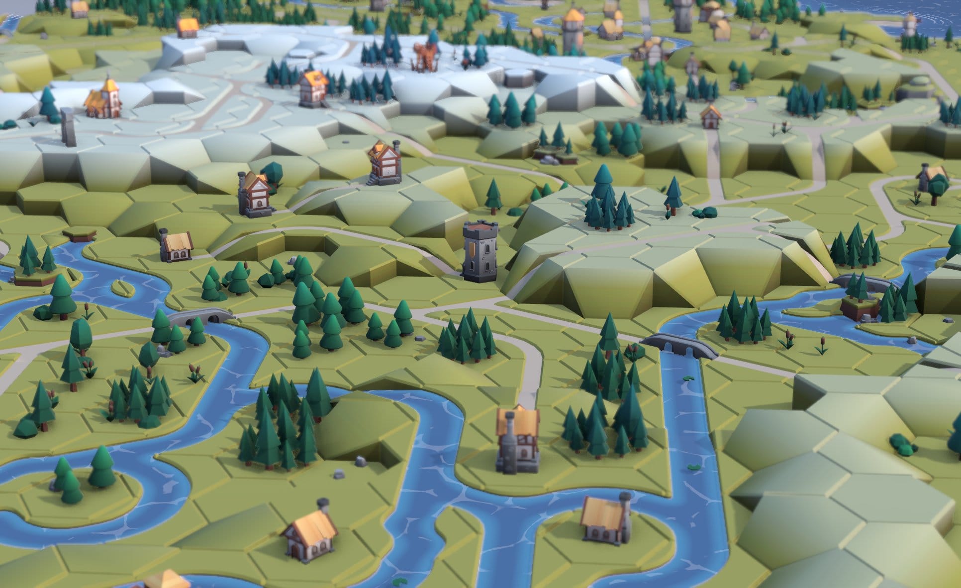
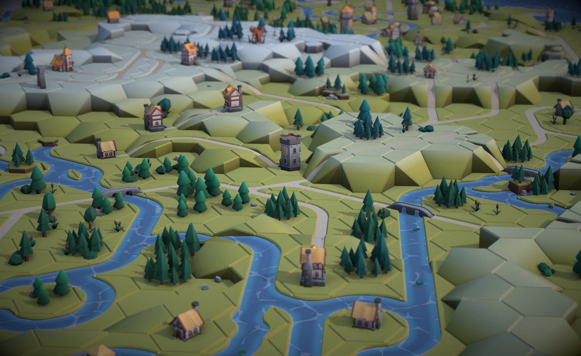
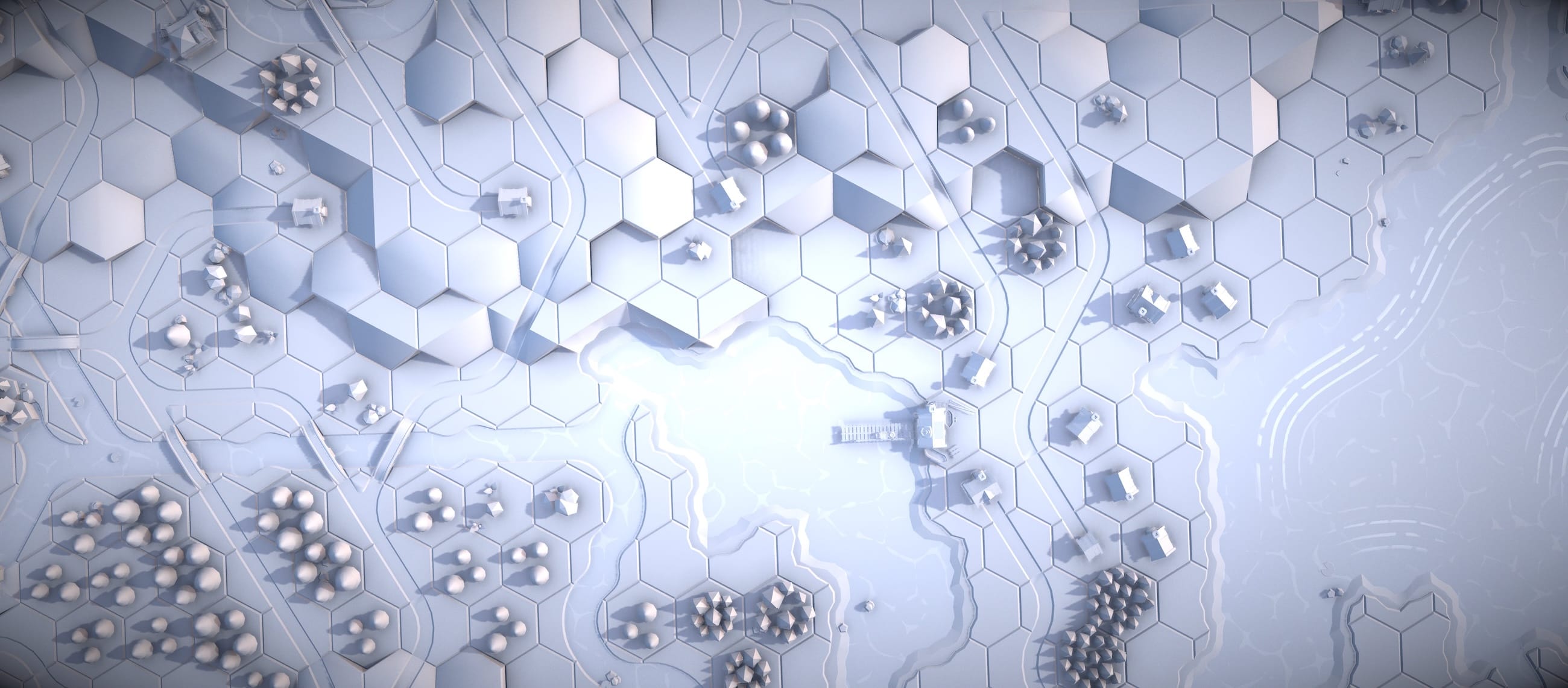
Every map is different. Every map is seeded and deterministic.

I've been obsessed with procedural maps since I was a kid rolling dice on the random dungeon tables in the AD&D Dungeon Master's Guide. There was something magical about it — you didn't design the dungeon, you discovered it, one room at a time, and the dice decided whether you got a treasure chamber or a dead end full of rats.

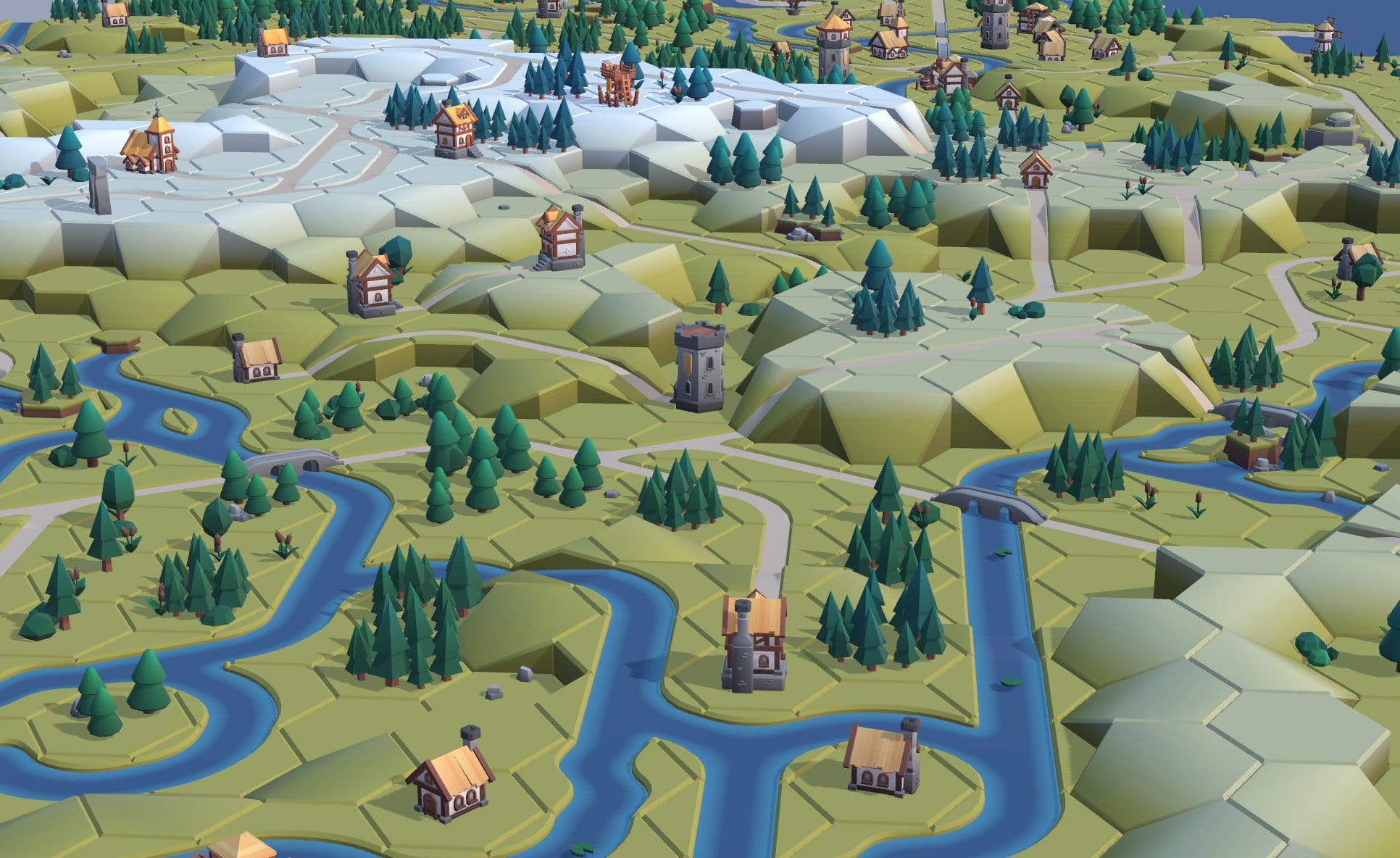
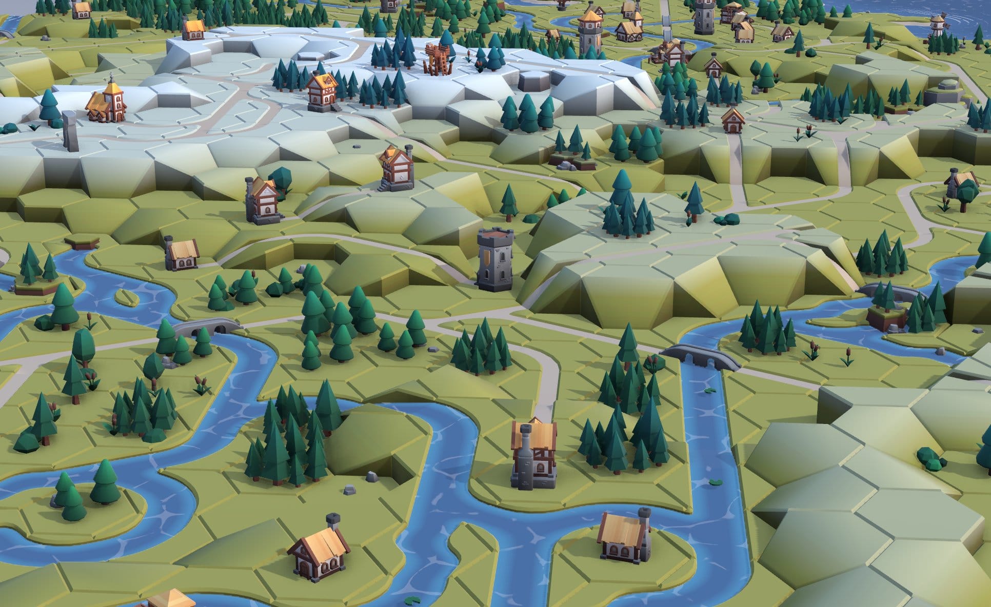
Years later, I decided to build my own map generator. It creates little medieval island worlds — with roads, rivers, coastlines, cliffs, forests, and villages — entirely procedurally. Built with Three.js WebGPU and TSL shaders, about 4,100 hex cells across 19 grids, generated in ~20 seconds.

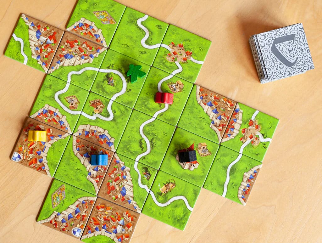
Carcassonne, but a Computer Does It

The core technique is Wave Function Collapse (WFC), an algorithm originally created by Maxim Gumin that's become a darling of procgen gamedev.

Hours of fun with map tiles.

If you've ever played Carcassonne, you already understand WFC. You have a stack of tiles and place them so everything lines up. Each tile has edges — grass, road, city. Adjacent tiles must have matching edges. A road edge must connect to another road edge. Grass must meet grass. The only difference is that the computer does it faster, and complains less when it gets stuck.

The twist: hex tiles have 6 edges instead of 4. That's 50% more constraints per tile, and the combinatorial explosion is real. Square WFC is well-trodden territory. Hex WFC is... less so.

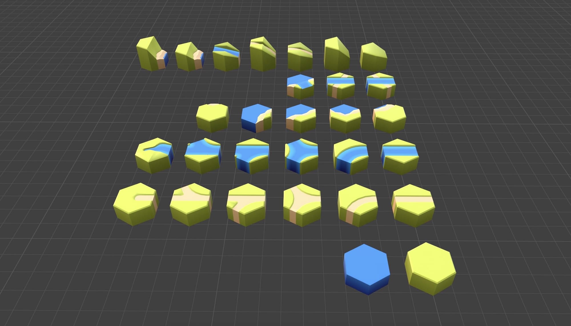
Tile Definitions

For this map there are 30 different tiles defining grass, water, roads, rivers, coasts and slopes. Each tile in the set has a definition which describes the terrain type of each of its 6 edges, plus a weight used for favoring some tiles over others.

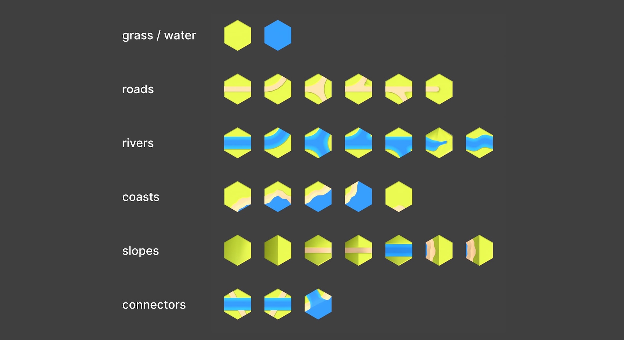
30 tile types, each with 6 rotations and 5 elevation levels. That's 900 possible states per cell.

For example this 3-way junction has 3 road edges and 3 grass edges. Tile definition:

{ name: 'ROAD_D', mesh: 'hex_road_D',
  edges: { NE: 'road', E: 'grass', SE: 'road', SW: 'grass', W: 'road', NW: 'grass' },
  weight: 2 }

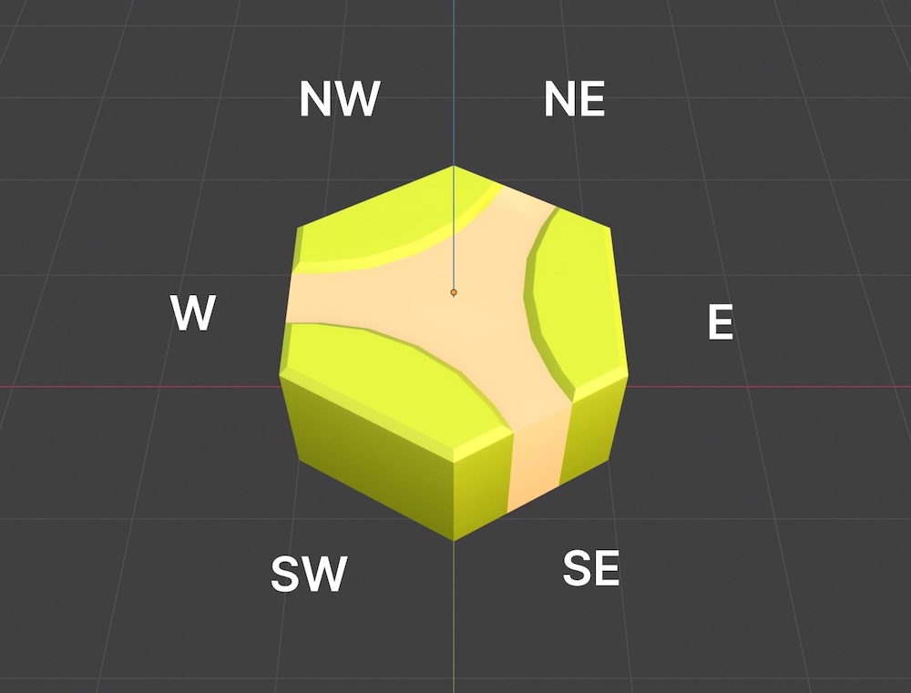
Each tile defines 6 edge types. Matching edges is the only rule.

How WFC Works

1. Start with chaos. Every cell on the grid begins as a superposition of all possible tiles — all 30 types, all 6 rotations, all 5 elevation levels. Pure possibility.
2. Collapse the most constrained cell. Pick the cell with the fewest remaining options (lowest entropy). Randomly choose one of its valid states.
3. Propagate. That choice constrains its neighbors. Remove any neighbor states whose edges don't match. This cascades outward — one collapse can eliminate hundreds of possibilities across the grid.
4. Repeat until every cell is solved — or you get stuck.

Getting stuck is the interesting part.

The Multi-Grid Problem

WFC is reliable for small grids. But as the grid gets bigger, the chance of painting yourself into a dead end goes up fast. A 217-cell hex grid almost never fails. A 4123-cell grid fails regularly.

The solution: modular WFC. Instead of one giant solve, the map is split into 19 hexagonal grids arranged in two rings around a center — about 4,100 cells total. Each grid is solved independently, but it has to match whatever tiles were already placed in neighboring grids. Those border tiles become fixed constraints.

And sometimes those constraints are simply incompatible. No amount of backtracking inside the current grid can fix a problem that was baked in by a neighbor. This is where I spent a lot of dev time.

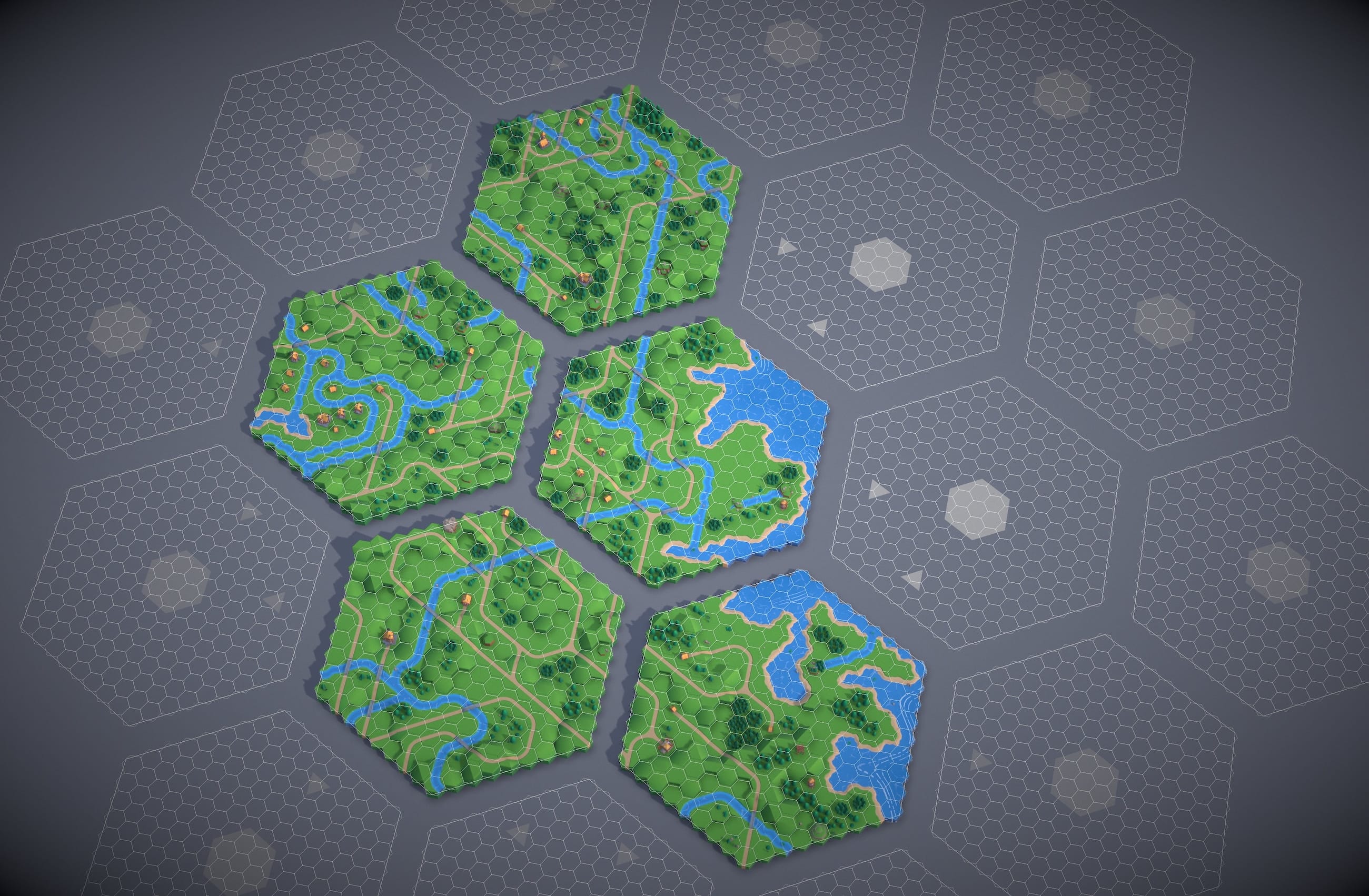
5 of 19 grids solved. Each grid is an independent WFC solve, constrained by its neighbors' border tiles.

Backtracking

Here's the dirty secret of WFC: it fails. A lot. You make a series of random choices, propagate constraints, and eventually back yourself into a corner where some cell has zero valid options left. Congratulations, the puzzle is unsolvable.

The textbook solution is backtracking — undo your last decision and try a different tile. My solver tracks every possibility it removes during propagation (a "trail" of deltas), so it can rewind cheaply without copying the entire grid state. It'll try up to 500 backtracks before giving up.

But backtracking alone isn't enough. The real problem is cross-grid boundaries.

The Recovery System

After many failed approaches, I landed on a layered recovery system:

Layer 1: Unfixing. During the initial constraint propagation, if a neighbor cell creates a contradiction, the solver converts it from a fixed constraint back into a solvable cell. Its own neighbors (two cells out — "anchors") become the new constraints. This is cheap and handles easy cases.

Layer 2: Local-WFC. If the main solve fails, the solver runs a mini-WFC on a small radius-2 region around the problem area — re-solving 19 cells in the overlap area to create a more compatible boundary. Up to 5 attempts, each targeting a different problem cell. Local-WFC was the breakthrough. Instead of trying to solve the impossible, go back and change the problem. The system even got up to ~86% success solving the entire map in one go.

Layer 3: Drop and hide. Last resort. Drop the offending neighbor cell entirely and place mountain tiles to cover the seams. Mountains are great — their cliff edges match anything, and they look intentional. Nobody questions a mountain.

Before: neighbor conflict blocks the solve

After: Local-WFC patches the boundary

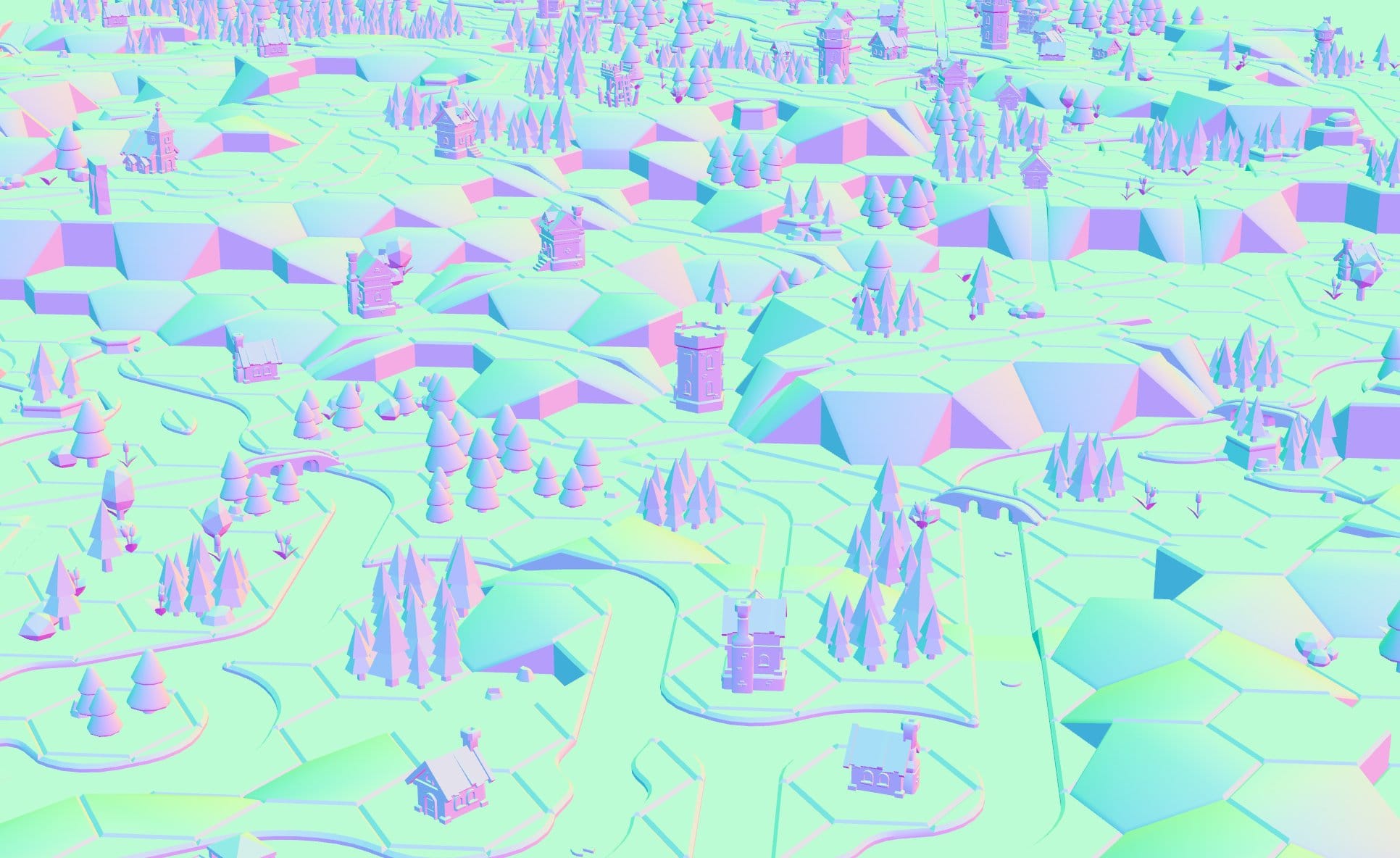
Debug mode showing the carnage. Purple = neighbor conflict. Red = broken tiles.

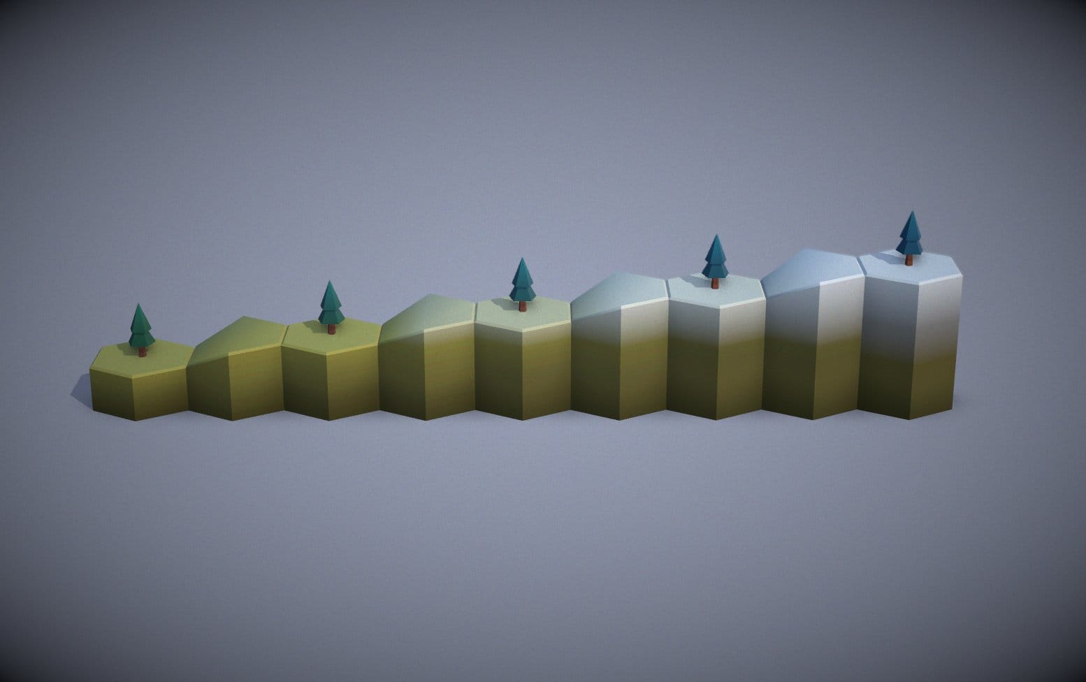
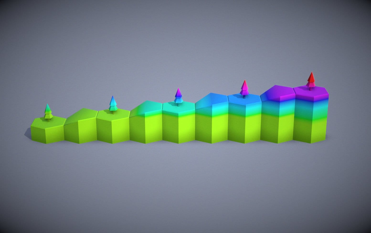
The Third Dimension

This map isn't flat — it has 5 levels of elevation. Ocean and Grass start at level 0, but slopes and cliffs can move up or down a level. Low slopes go up 1 level, high slopes go up 2 levels. A road tile at level 3 needs to connect to another road tile at level 3, or a slope tile that transitions between levels. Get it wrong and you end up with roads that dead-end into cliff faces or rivers flowing uphill into the sky. The elevation axis turns a 2D constraint problem into a 3D one, and it's where a lot of the tile variety (and a lot of the solver failures) comes from.

Natural

Debug Colors

Elevation colors.

Tiles are colored with a node-based PBR material - MeshPhysicalNodeMaterial - with a custom TSL color node. Each tile's elevation is encoded in the instance color, which the shader uses to blend between two palette textures — low ground gets summer colors, high ground gets winter.

Hex Coordinates: Surprisingly Weird

Hex math is weird. Since there are 6 directions instead of 4, there's no simple mapping between hex positions and 2D x,y coordinates. The naive approach is offset coordinates — numbering cells left-to-right, top-to-bottom like a regular grid. This works until you need to find neighbors, compute distances, or do anything involving directions. Then it gets confusing fast, with different formulas for odd and even rows.

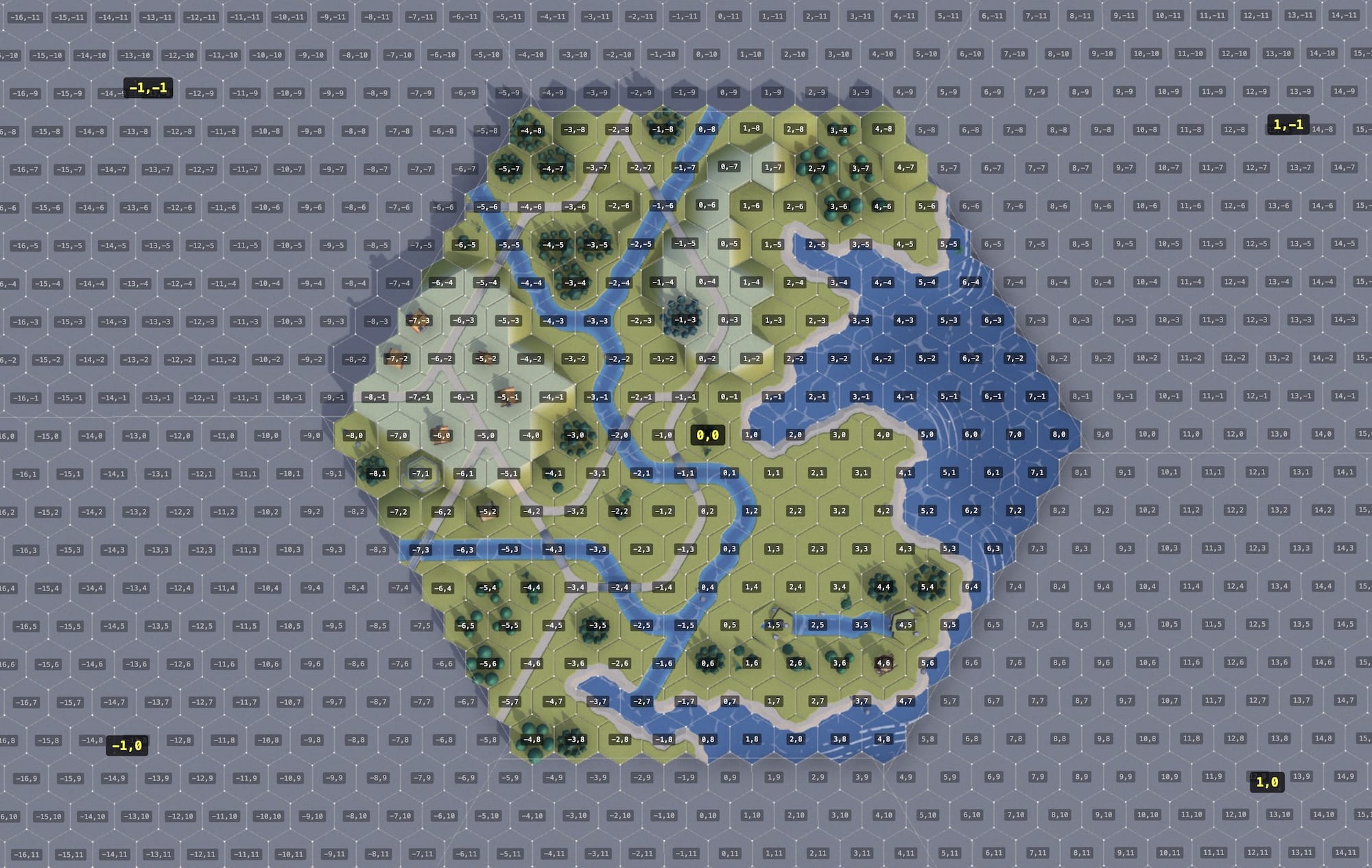
Offset coordinates: simple until you need to do anything useful with them.

The better approach: cube coordinates (q, r, s where s = -q-r). It's a 3D coordinate system for the three hex axes. Neighbor finding becomes trivial — just add or subtract 1 from two coordinates.

The good news is that WFC doesn't really care about geometry. It's concerned with which edges match which — it's essentially a graph problem. The hex coordinates only matter for rendering and for the multi-grid layout, where the 19 grids are themselves arranged as a hex-of-hexes with their own offset positions.

If you've ever worked with hex grids, you owe Amit Patel at Red Blob Games a debt of gratitude. His hex grid guide is the definitive reference.

Trees, Buildings, and Why Not Everything Should Be WFC

Early on, I tried using WFC for tree and building placement. Bad idea. WFC is great at local edge matching but terrible at large-scale patterns. You'd get trees scattered randomly instead of clustered into forests, or buildings spread evenly instead of gathered into villages.

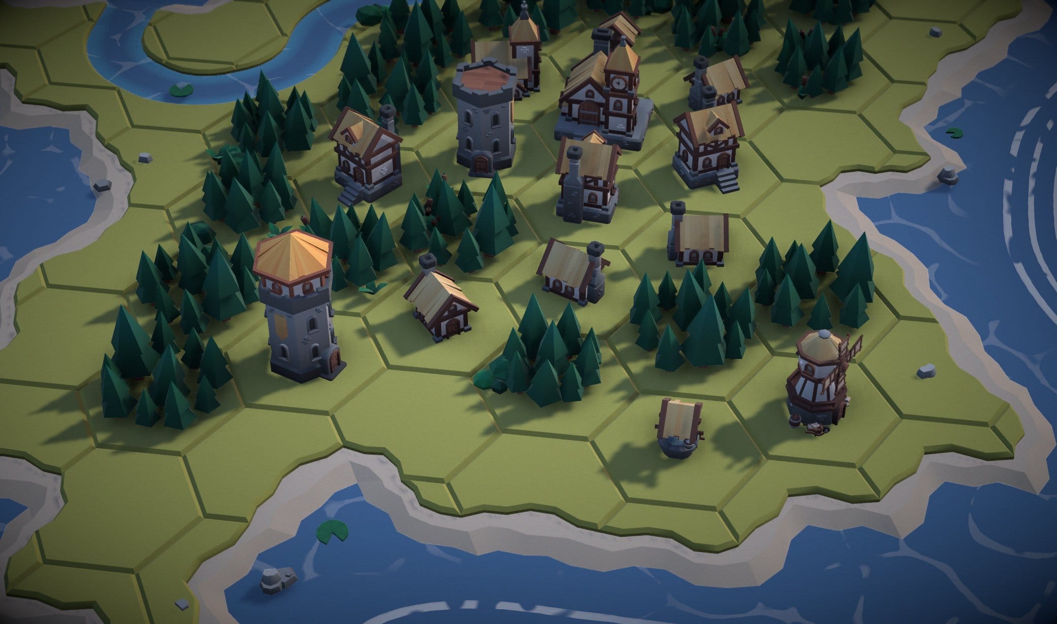
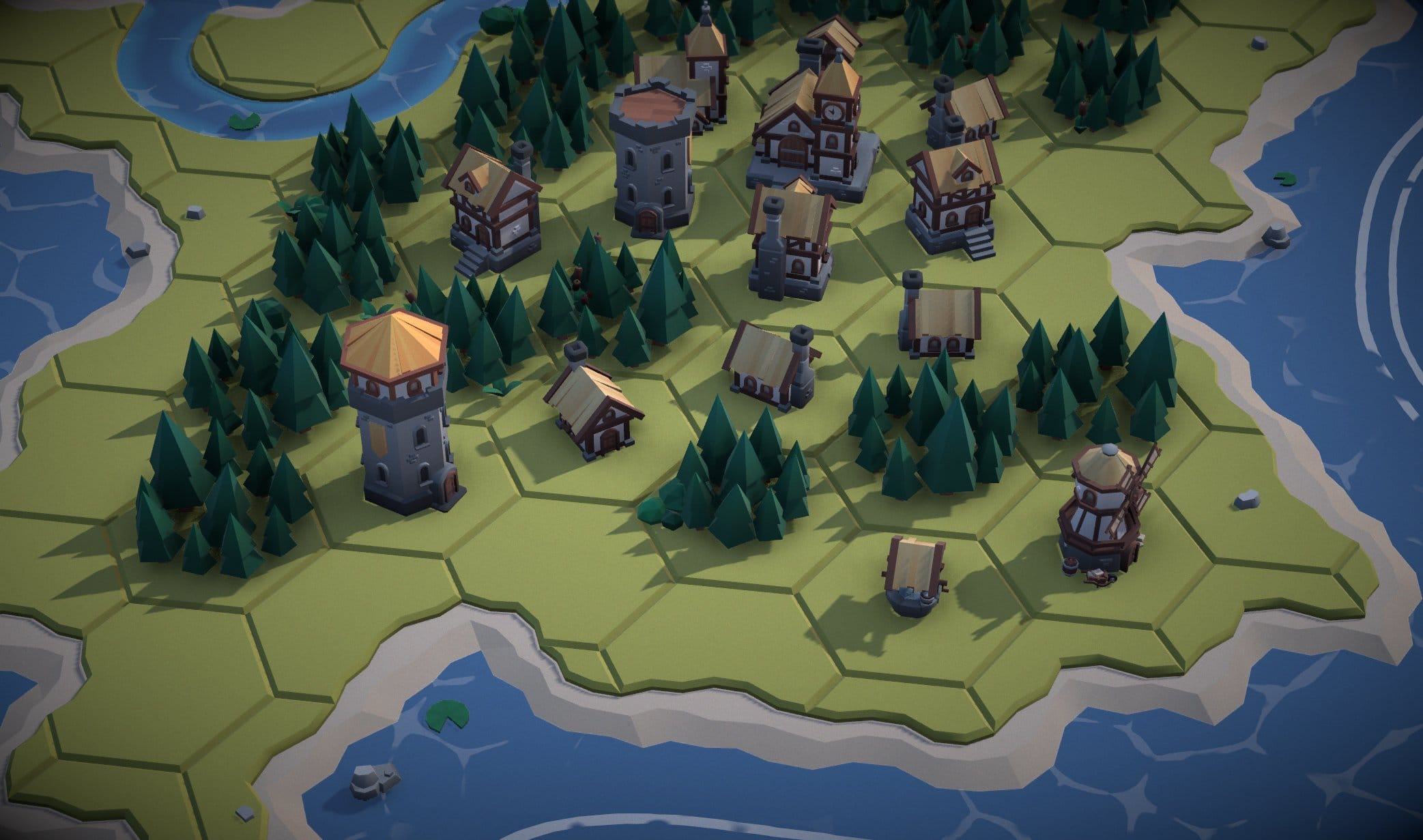
The solution: good old Perlin noise. A global noise field determines tree density and building placement, completely separate from WFC. Areas where the noise is above a threshold get trees; slightly different noise drives buildings. This gives you organic clustering — forests, clearings, villages — that WFC could never produce. I also used some additional logic to place buildings at the end of roads, ports and windmills on coasts, henges on hilltops etc.

WFC handles the terrain. Noise handles the decorations. Each tool does what it's good at.

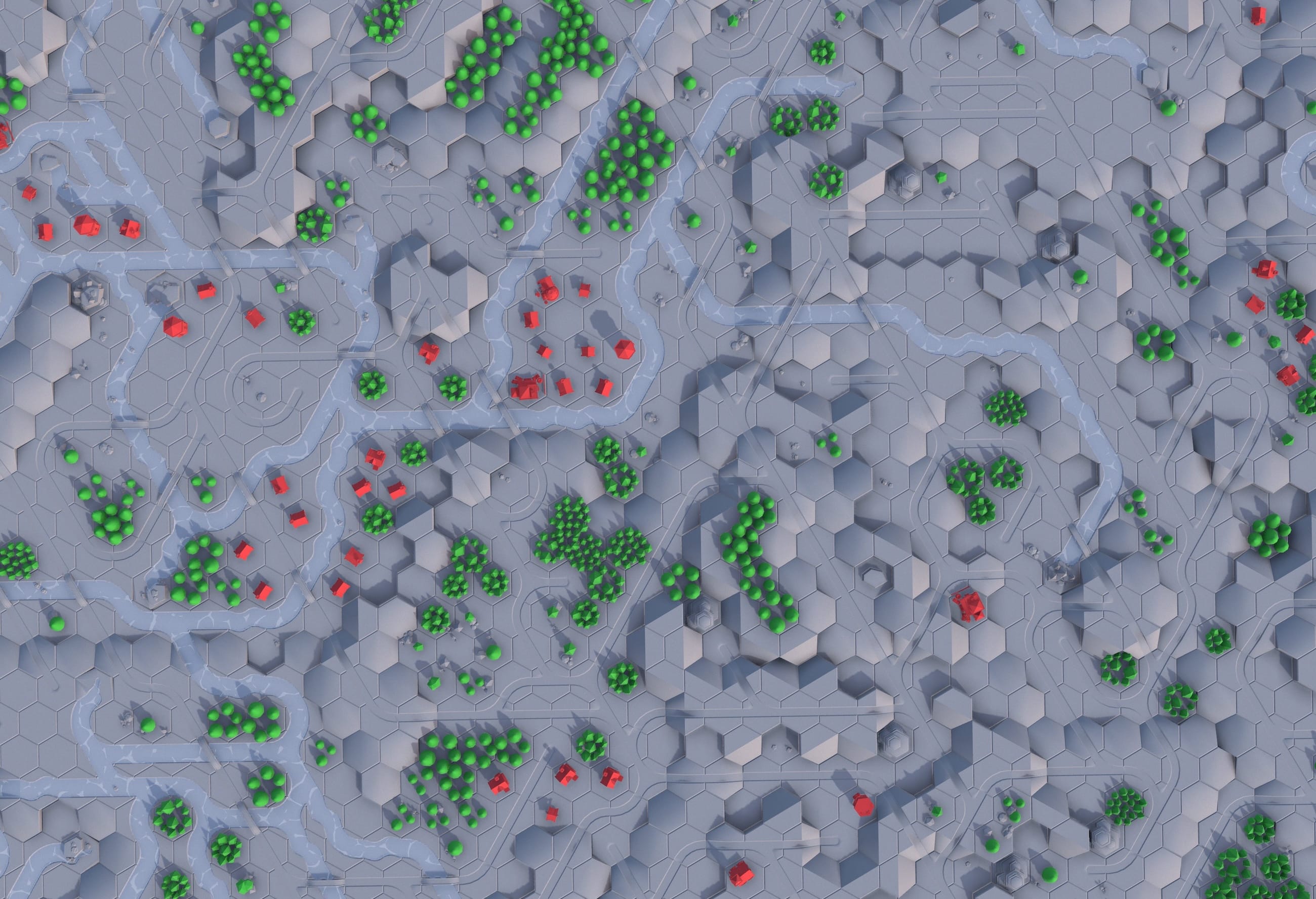
Buildings cluster along roads. Forests form natural groups. None of this is WFC — it's all noise-based placement.

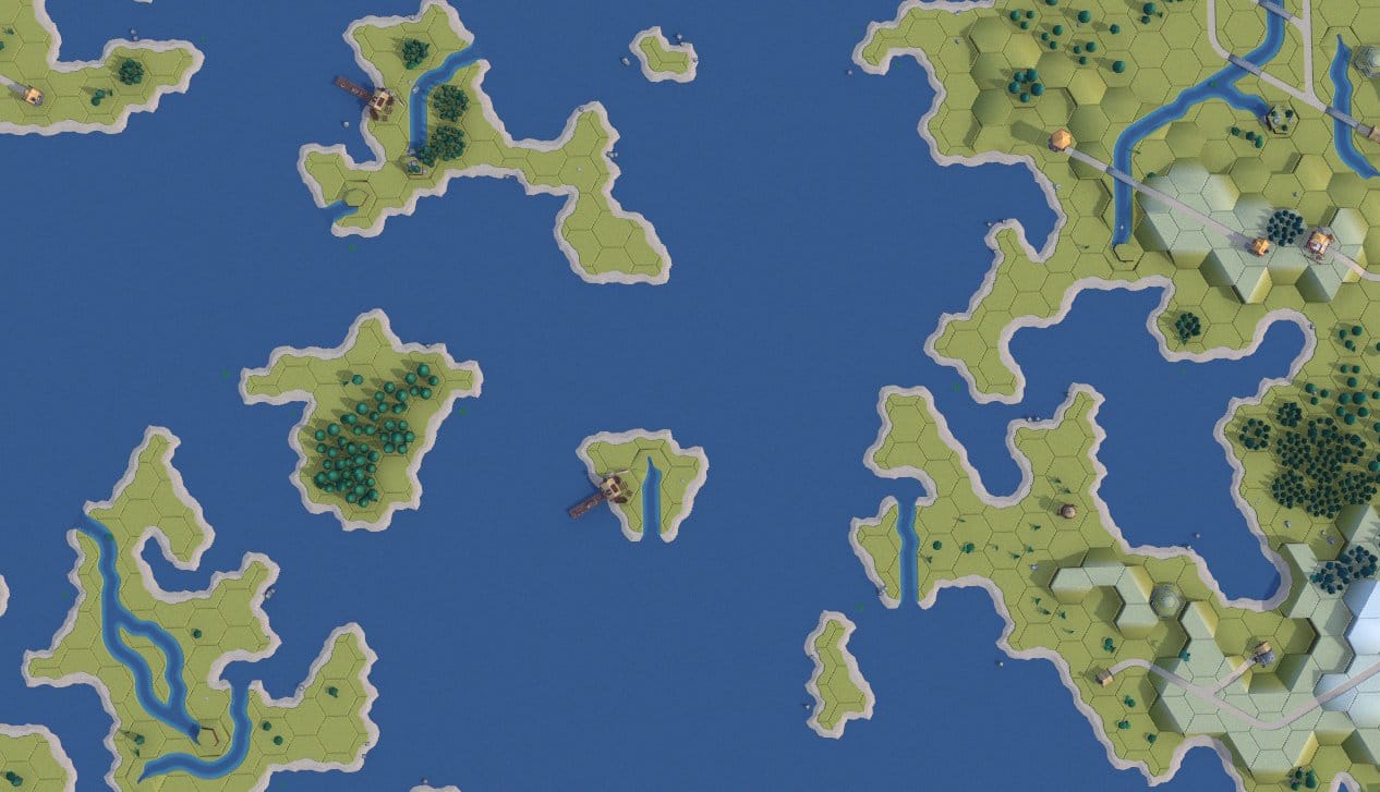
Water: Harder Than It Looks

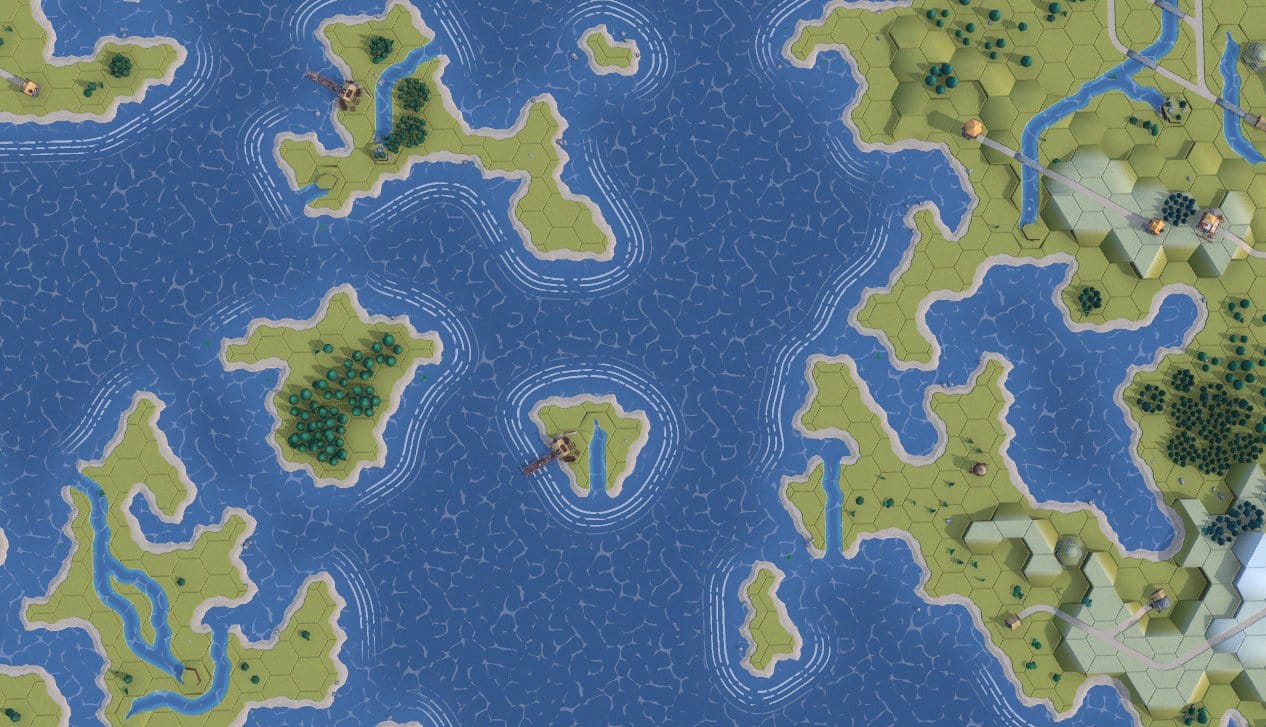
Water effects were the hardest visual problem to solve. The ocean isn't just a blue plane — it has animated caustic sparkles and coastal waves that emanate from shorelines.

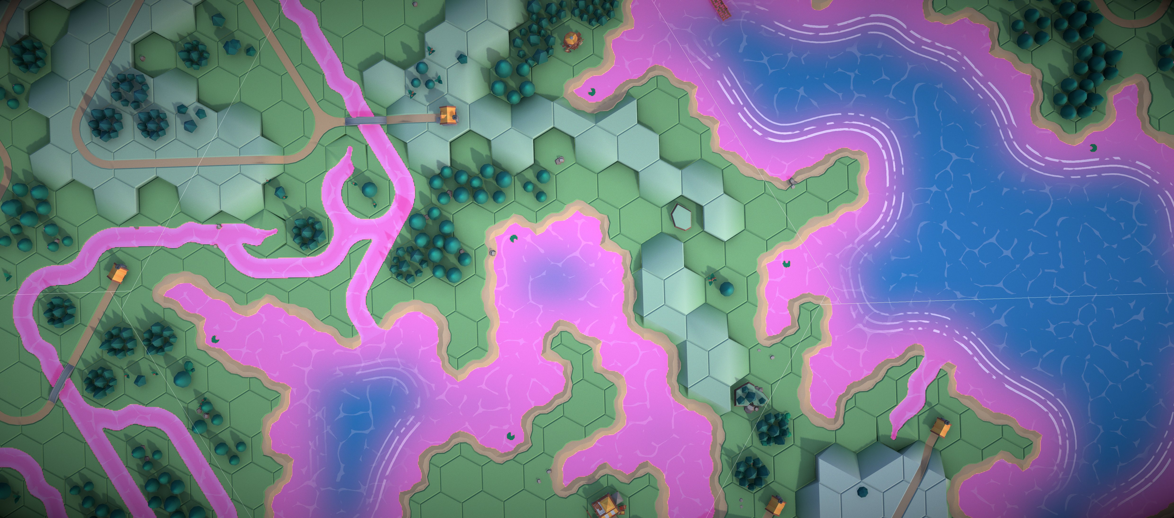
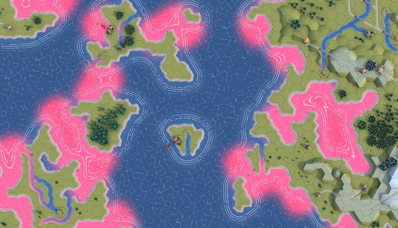
Pink is the best debug color.

Sparkles

I wanted that 'Zelda: The Wind Waker' cartoon shimmer on the water surface. Originally I tried generating caustics procedurally with four layers of Voronoi noise. This turned out to be very GPU heavy and did not look great. The solution was sampling a small scrolling caustic texture with a simple noise mask, which looks way better and is super cheap. Sometimes the easy solution is the correct solution.

Coast Waves

Waves are sine bands that radiate outward from coastlines, inspired by Bad North's gorgeous shoreline effect. To know "how far from the coast" each pixel is, the system renders a coast mask — a top down orthographic render of the entire map with white for land and black for water — then dilates and blurs it into a gradient. The wave shader reads this gradient to place animated sine bands at regular distance intervals, with noise to break up the pattern.

Flat blue plane

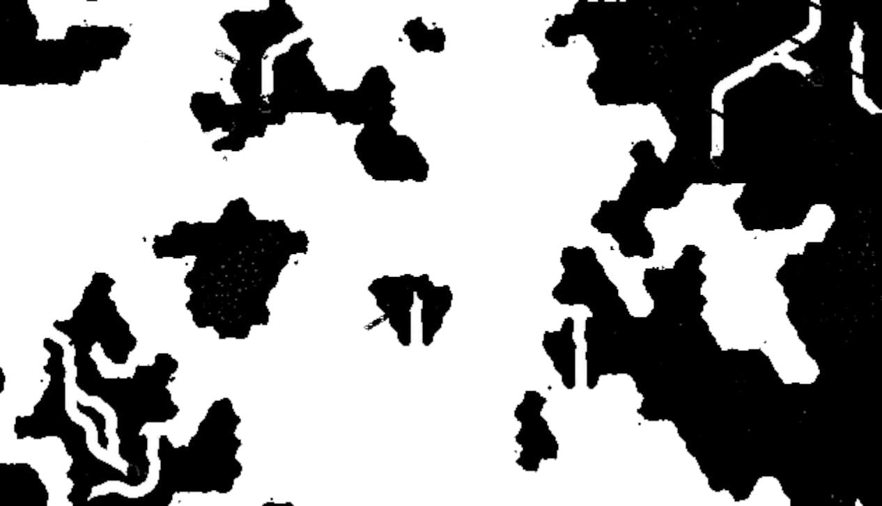Water mask

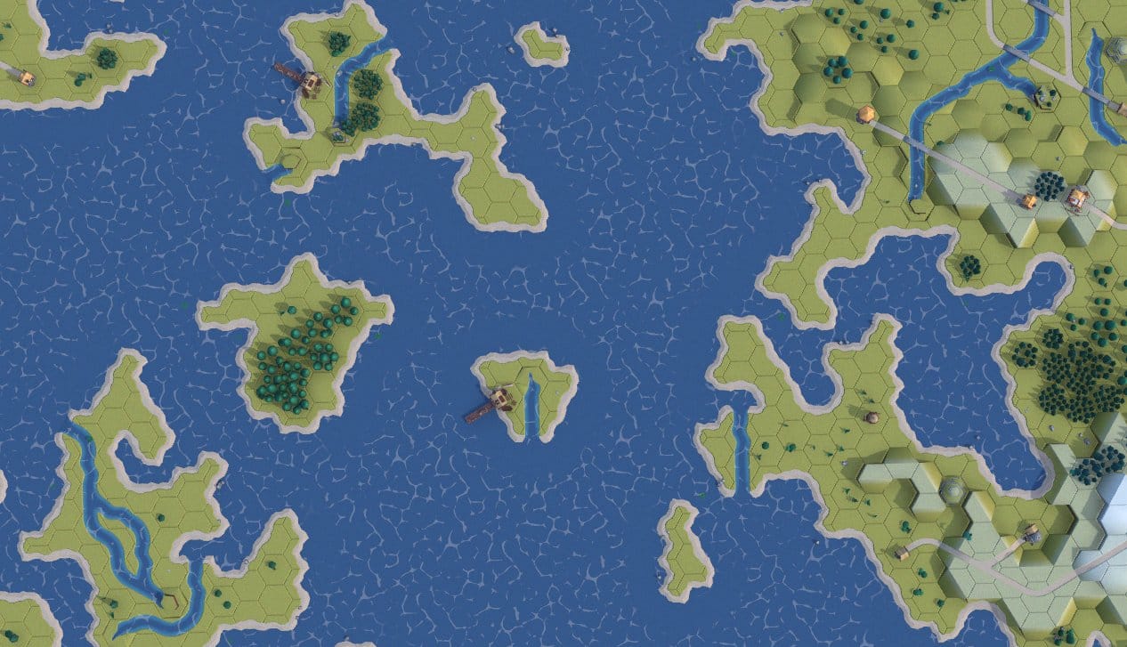Caustic sparkles

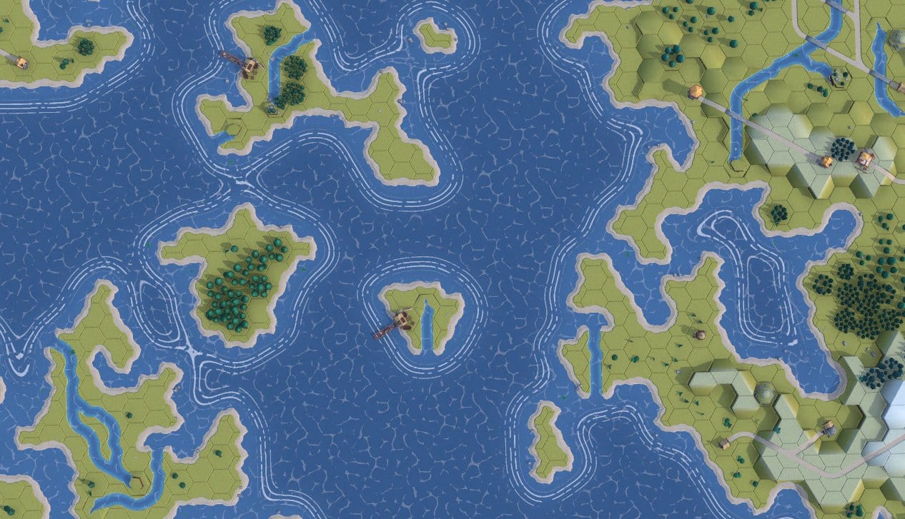Coast waves fat in coves

Surroundedness mask

Final water

Building up the water effect layer by layer.

The Cove Problem

This worked great on straight coastlines. In concave coves and inlets, the wave lines got thick and ugly. The blur-based gradient spreads the same value range over a wider physical area in coves, stretching the wave bands out.

I tried multiple fixes:

• Screen-space derivatives to detect gradient stretching — worked at one zoom level, broke at others.
• Texture-space gradient magnitude to detect opposing coast edges canceling out — only detected narrow rivers, not actual problem coves.
• Extra dilation passes — affected straight coasts too.

The fundamental issue: blur encodes "how much land is nearby," not "how far is the nearest coast edge." These are different questions, and no amount of post-processing the blur can extract true distance.

The solve was to do a CPU-side "surroundedness" probe that checks each water cell's neighbors to detect coves, writing a separate mask texture that thins the waves in enclosed areas. It's kind of a hack but it works and the wave edges thin out nicely at the edges.

Making Tiles in Blender

The 3D tile assets come from KayKit's fantastic low-poly Medieval Hexagon pack. But it was missing some key connectors needed for a sub-complete tileset, so I dusted off my Blender skills and built new tiles: sloping rivers, river dead-ends, river-to-coast connectors, and several cliff edge variants.

The key constraint: every tile is exactly 2 world units wide, and edge types must align perfectly at the hex boundaries. Getting UVs right means the texture atlas maps correctly across tile seams. A misaligned UV by even a few pixels creates a visible seam line that breaks the illusion.

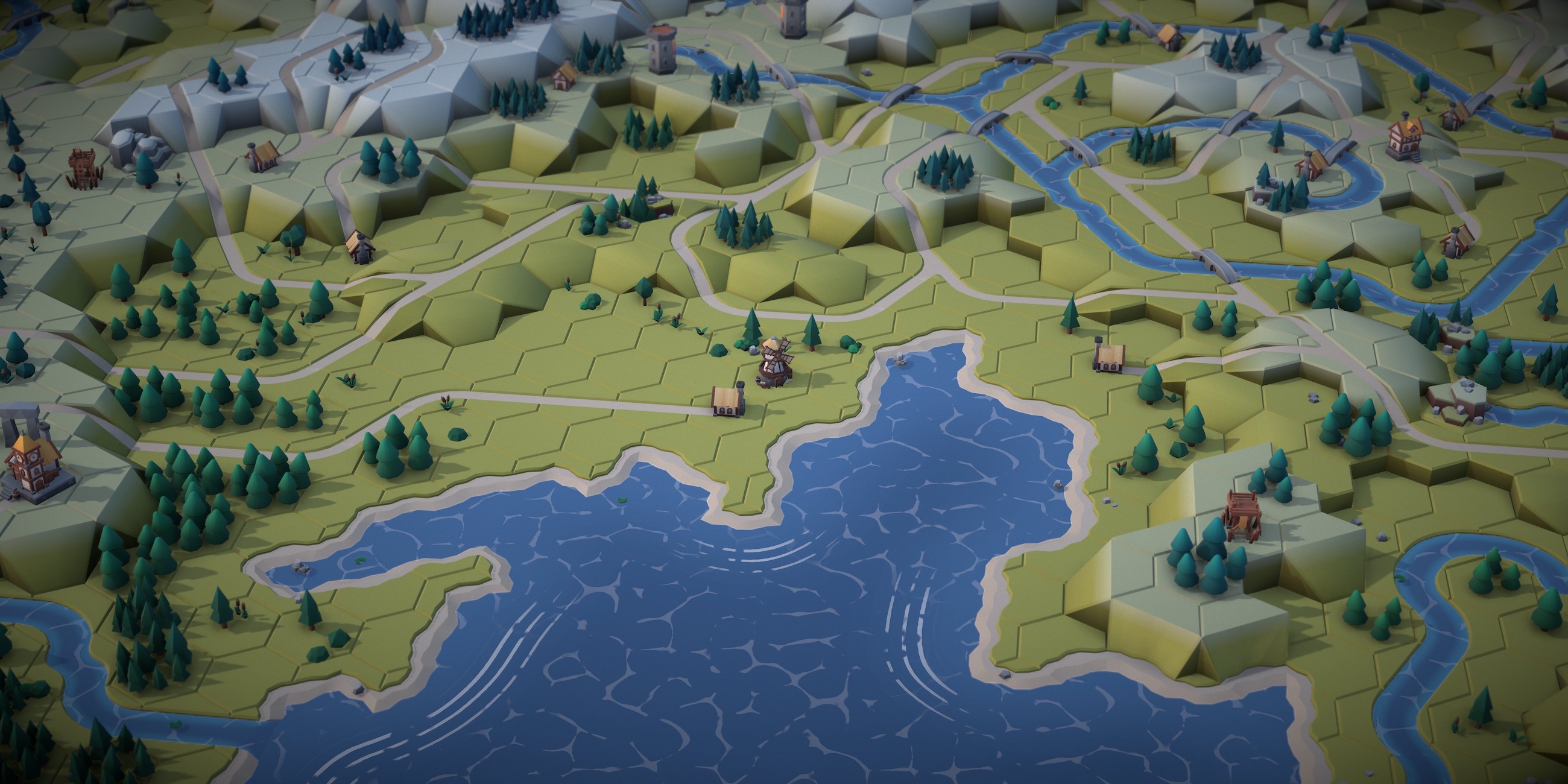
Making It Pretty

The algorithm gets you a valid map. Making it look like a place you'd want to visit is a whole separate problem.

WebGPU and TSL Shaders

The renderer is Three.js with WebGPU and TSL (Three.js Shading Language) — the new node-based shader system that replaces raw GLSL. All the custom visual effects are written in TSL, which reads like a slightly alien dialect of JavaScript that runs on your GPU.

The Post-Processing Stack

The raw render looks... fine. Flat. Like a board game photographed under fluorescent lights. The post-processing pipeline is what gives it atmosphere:

1. GTAO Ambient Occlusion — darkens crevices between tiles, around buildings and trees. This makes everything feel more solid. The AO result is denoised to reduce speckling. This runs at half resolution since AO and denoising is expensive.
2. Depth of Field — tilt-shift blur based on camera distance gives it that miniature/diorama feel. The DOF focal length scales with the camera zoom to give more DOF when zoomed in.
3. Vignette + Film Grain — subtle edge darkening and noise. Just enough to feel analog.

Normals

AO

Raw render

AO Composite

DOF

Vignette and Grain

Post-processing. AO, depth of field and grain do a lot of heavy lifting.

Dynamic Shadow Maps

The shadow map frustum is fitted to the camera view every frame. The visible area is projected into the light's coordinate system to compute the tightest possible bounding box, so no shadow map texels are wasted on off-screen geometry. Zoomed out, shadows cover the whole map at lower resolution. Zoom in, and the shadow map tightens to give you crisp, detailed shadows on individual tiles. This prevents blocky shadow artifacts when you zoom in.

Fixed shadow map

Dynamic shadow map

Dynamic frustum for crisp detail.

Optimizations

The complete map has thousands of tiles and decorations. Drawing each one individually would kill the frame rate. The solution is two-fold:

BatchedMesh — each hex grid gets 2 BatchedMeshes: one for tiles, one for decorations. The beauty of a BatchedMesh is that each mesh can have separate geometry and transforms, but they all render in a single draw call. The GPU handles per-instance transforms and geometry offsets, so CPU cost is essentially zero after setup.

The whole scene renders in a handful of draw calls regardless of map complexity. That means the base render is cheap, so you can spend your GPU budget on AO, DoF, and color grading instead.

One Shared Material — every mesh in the scene shares a single material. The Mesh UVs map into a small palette texture, so they all pull their color from the same image, like a shared paint-by-numbers sheet. One material means zero shader state switches between draw calls, so the GPU can blast through 38 BatchedMeshes without stalling.

The result: 4,100+ cells, 38 BatchedMeshes, and the whole thing renders at 60fps on desktop and mobile.

Snow day.

Summary

No dice required this time — but the feeling is the same. You hit a button, the map builds itself, and you discover what the algorithm decided to put there. It's super satisfying to see the road and river systems matching up perfectly. Every time it's different, and every time I find myself exploring for a while. The kid rolling dice on the dungeon tables would be into this.

The Numbers

30 tile types

19 hexagonal grids

~4,100 total cells

2 draw calls per grid

500 max backtracks

5 Local-WFC attempts

~20s to build all grids

100% success rate (500 runs)

Tech Stack

• Three.js r183 with WebGPU renderer
• TSL (Three.js Shading Language) for all custom shaders
• Web Workers for off-thread WFC solving
• Vite for builds
• BatchedMesh for efficient tile rendering (one draw call)
• Seeded RNG for deterministic, reproducible maps

Try It

Play with the live demo — click the hex buttons to expand the map, or hit 'Build All' to generate the whole thing. There's a full GUI panel with 50+ tweakable parameters if you want to mess with the lighting, color grading, water effects, and WFC settings.

Full source code on GitHub

About Me

I'm Felix Turner, a creative developer and founder of Airtight Interactive. I build interactive visual experiments, WebGL/WebGPU experiences, and generative art.

Twitter · Bluesky