Elon Litman

Borges wrote a story about a man named Funes who, after a horseback accident, acquires the ability to perceive and remember everything. Every leaf on every tree. Every ripple on every stream at every moment. He is the perfect empiricist. Infinite data, infinite recall, infinite resolution. And he cannot think. Because thinking, as Borges understood, requires forgetting. Funes could reconstruct entire days from memory but could not understand why the dog at 3:14, seen from the side, should be called the same thing as the dog at 3:15, seen from the front.

_I suspect [that Funes] was not very good at thinking. To think is to ignore (or forget) differences, to generalize, to abstract. In the teeming world of Ireneo Funes there was nothing but particulars._Jorge Luis Borges, "Funes the Memorious," in Ficciones (1944).

Later in the story, Borges conjures Locke, who in the seventeenth century postulated an impossible language in which each individual thing, each stone, each bird and each branch, would have its own name. Funes projected an analogous language but discarded it because it seemed too general to him, too ambiguous. Deep learning theory has built Locke's language and is well on its way to Funes'. More parameters. More data. Deeper networks. More compute. Uniform convergence people, optimization people, NTK people, PAC-Bayes people, stability people, mean-field people, all working on the same problem, none of them speaking the same language, each proving bounds under assumptions that are vacuous under each other's assumptions.

Deep learning alchemy today is where chemistry was before Lavoisier: a practice that works, built on a theory that doesn't. Everyone agrees this is a problem. Few believe it is a solvable one. At the Diffusion Group at Stanford, we have been trying for some time to answer this question, which most of our colleagues consider premature and quixotic: why does deep learning work? We think we have an answer.

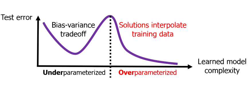
But first, to see why the question is hard, start with what classical theory predicts. Classical statistical learning theory posits the bias-variance tradeoff: too simple and you underfit the data, too expressive and you overfit. Deep neural networks are highly expressive and overparameterized—they have far more parameters than data points; they can shatter any possible labeling of the data. During training, the network interpolates the training data perfectly, including all noise, achieving zero error. Surely, the test error should be catastrophic.Zhang et al., "Understanding Deep Learning (Still) Requires Rethinking Generalization," Communications of the ACM 64, no. 3 (2021). The original 2017 version demonstrated that standard architectures can memorize random labels, establishing that classical capacity-based explanations of generalization are insufficient. But then, the test error…

is also very low.

This is called benign overfitting. It violates the most basic intuition in statistical learning theory.Bartlett et al., "Benign Overfitting in Linear Regression," PNAS 117, no. 48 (2020). You fit the training data exactly, so presumably the noise must have been destroyed, or rendered harmless in some form.

Trying to visualize the bias-variance tradeoff with neural networks doesn't yield the expected U-shaped curve, but instead shows double descent. Test error goes up as model complexity increases, then comes back down past the interpolation threshold.Belkin et al., "Reconciling Modern Machine Learning Practice and the Bias-Variance Trade-off," PNAS 116, no. 32 (2019). At the exact moment the network gains the capacity to memorize everything, it begins to generalize.

Gradient descent, given infinitely many solutions that interpolate the data, picks ones that generalize (usually low \(\ell_2\)-norm, low nuclear norm, approximately low-rank). This is called implicit bias.Gunasekar et al., "Implicit Regularization in Matrix Factorization," NeurIPS (2017), and Soudry et al., "The Implicit Bias of Gradient Descent on Separable Data," JMLR 19 (2018).

Lastly, in cases where the data-generating distribution is highly structured and the network doesn't possess the right inductive bias, the network memorizes the training set, then much later, hundreds of thousands of steps later, suddenly generalizes. This is _grokking._Power et al., "Grokking: Generalization Beyond Overfitting on Small Algorithmic Datasets," arXiv:2201.02177 (2022).

Our explanation is available via preprint here.Litman & Guo, "A Theory of Generalization in Deep Learning," arXiv:2605.01172. It comes with proofs, experiments, and an algorithm that allows you to train on the population risk of any model, loss function, and dataset.

The Theory

The standard approach treats a neural network as a point in a hypothesis class, attempting to bound its complexity across billions of parameters. We propose a radical Vereinfachung: abandoning the parameter space entirely. Instead, we analyze the network as a dynamical system strictly in output space, focusing on how predictions evolve and where error flows. Stack all training outputs into a vector \(U_S \in \mathbb{R}^{np}\). Form the Jacobian \(J_S = D_w U_S\), the matrix of partial derivatives of every output with respect to every parameter. The object that governs everything is the empirical Neural Tangent Kernel (eNTK):Jacot et al., "Neural Tangent Kernel: Convergence and Generalization in Neural Networks," NeurIPS (2018).

$$K_{SS}(w) = J_S(w) J_S(w)^\top$$

A matrix that tells you, for every pair of training points, how much a gradient step on one affects the prediction on the other. Under gradient flow, the training outputs and their gradient evolve as

$$\partial_t u = -K_{SS} g$$

$$\partial_t g = -B K_{SS} g$$

Where \(g = \nabla \Phi_S(u)\) is the output gradient and \(B = \nabla^2 \Phi_S(u)\) is the loss Hessian. The test outputs evolve in parallel through the cross-kernel \(K_{QS} = J_Q J_S^\top\):

$$\partial_t U_Q = -K_{QS} g$$

This holds for any differentiable architecture and any convex loss, without any infinite-width or depth limit. The loss itself dissipates as

$$\frac{d}{dt}\Phi_S(u(t)) = -g(t)^\top K_{SS}(t) \, g(t) = -\|J_S^\top g\|_2^2$$

Loss decreases at a rate set by the kernel. Decompose \(g\) along eigenvectors \(v_i\) of \(K_{SS}\) with eigenvalues \(\lambda_i\). For squared loss the residual \(r = u - y\) obeys \(\partial_t r = -M(t)r\) where \(M = K_{SS}/n\), so the component along \(v_i\) decays as \(e^{-\lambda_i t / n}\). A mode with eigenvalue \(10\lambda\) is learned ten times faster. On any finite training horizon, modes below some eigenvalue threshold have barely moved. Given infinite time, all modes are interpolated, noise included.

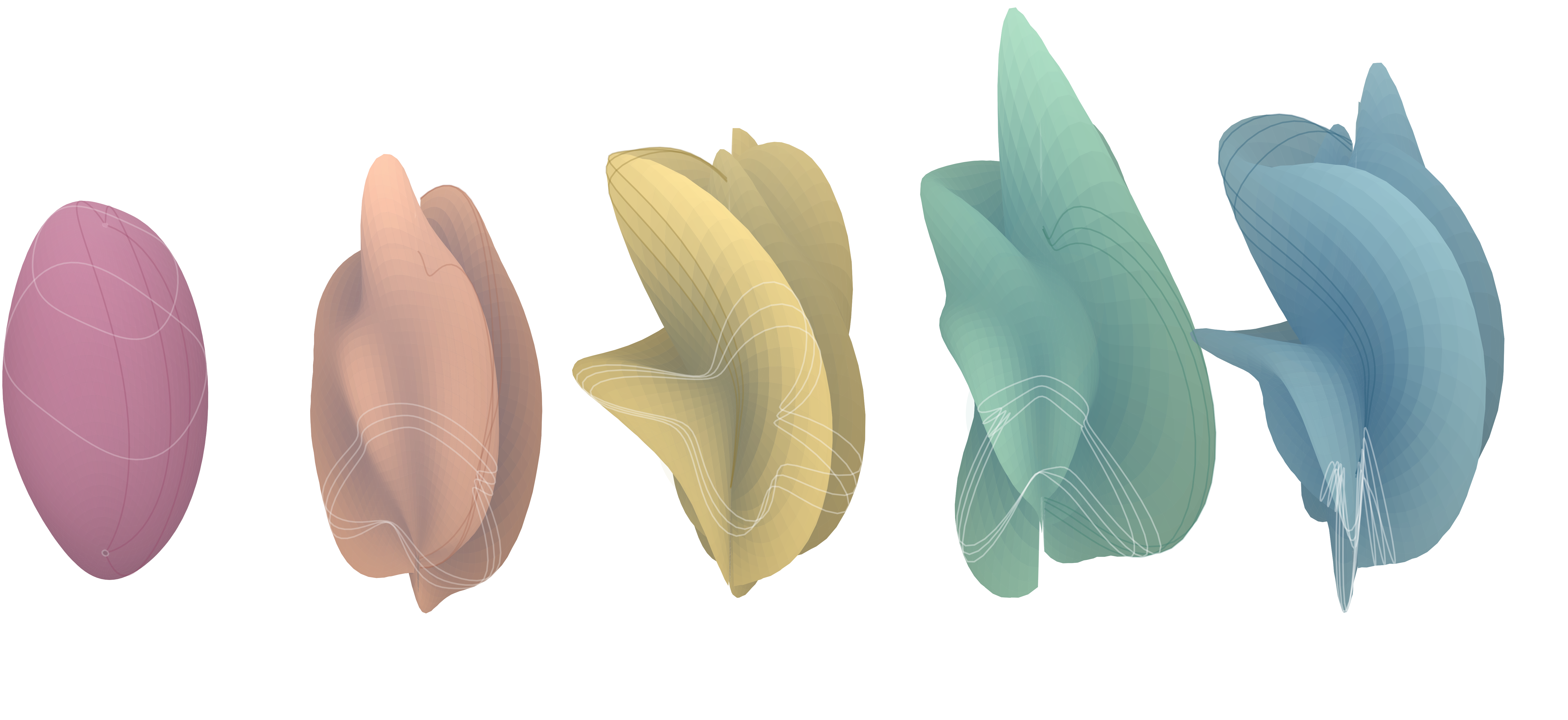
In the feature learning regime, the kernel is not fixed. As the parameters move, the eigenvectors rotate and the eigenvalues shift, so signal and noise get rearranged. Here is the kernel rotating (plotted by centering and normalizing its Gram matrix, extracting eigenstructure changes relative to initialization, mapping those changes into a shaded deformed surface):

To capture the cumulative effect of the entire training trajectory, we take the time integral of the eNTK:

$$\mathcal{W}_S(s,T) = \int_s^T P_g(\tau,s)^\top K_{SS}(\tau) P_g(\tau,s) \, d\tau$$

where \(P_g\) is the propagator of the gradient ODE. The eigenvalue of \(\mathcal{W}_S\) along direction \(\psi_j\) is the total integrated squared reachability of that direction over the entire training window:

$$\lambda_j = \int_s^T \|J_S(\tau)^\top P_g(\tau,s) \psi_j\|_2^2 \, d\tau$$

Directions with large \(\lambda_j\) are where training dissipated loss. This is the signal channel, \(\text{range}(\mathcal{W}_S)\). Directions with \(\lambda_j = 0\) are where training dissipated nothing. This is the reservoir, \(\ker(\mathcal{W}_S)\).

Now define the test transfer operator

$$G_Q(T,s) = \int_s^T K_{QS}(\tau) P_g(\tau,s) \, d\tau$$

which propagates the initial gradient to test displacement: \(U_Q(T) - U_Q(s) = -G\,g(s)\). We show that \(G\) vanishes on the reservoir. \(\ker \mathcal{W} \subseteq \ker G\). Thus, whatever the network memorized in the reservoir is invisible at test time. The point of overparameterization, of depth, of inductive bias, is to give the kernel a spectrum that puts signal in the channel and noise in the reservoir.

The Field, Reinterpreted

This theory unifies the major puzzles of deep learning theory under one mechanism.

Benign overfitting is noise sitting in the reservoir at interpolation. The network memorized the noise in the train set, but the noise is in the reservoir \(\ker \mathcal{W}_S\), which is test-invisible. It doesn't matter. As a pedagogical sidenote: yes, I know that in highly overparameterized networks this is technically a soft reservoir of near-zero eigenvalues rather than strictly a mathematical null space, but treating it as a hard boundary is the best way to build intuition for why that trapped noise disappears at test time.

Double descent is noise moving between the signal channel and the reservoir as model capacity sweeps across interpolation. At the interpolation threshold, noise briefly enters the signal channel and test error spikes. Past it, the noise gets absorbed back into the reservoir.

Implicit bias is the spectral schedule of \(\mathcal{W}_S(t)\) filling the signal channel from the largest kernel eigenvalue down. Gradient flow learns parsimonious, high-mobility modes first and low-mobility modes last. By strictly confining its test predictions to this accumulated signal channel, the network acts as a Moore-Penrose pseudo-inverse over the realized path, effectively finding the minimum-norm solution in the dynamic feature space rather than the static parameter space.

Grokking is signal migrating from the reservoir into the signal channel as the kernel evolves over training. The network memorizes first (fast noise-fitting modes saturate early), then generalizes later (slow signal modes finally enter the signal channel).

By the way: the same operators that explain generalization also give you a way to train directly on population risk. Treating each training point in a minibatch as a one-point held-out test set against the rest and localizing to a single optimizer step collapses the operator expression to a per-parameter rule: update parameter \(k\) if and only if

$$\mu_k^2 > \frac{\sigma_k^2}{b-1}$$

That is, if the batch signal on a parameter exceeds its leave-one-out noise, update it; if not, skip it. This is a one-line change to Adam that accelerates grokking by \(5 \times\), suppresses memorization in PINNs, and improves DPO fine-tuning, eliminating the need for validation sets entirely.

What the Future Holds

The math indicates several exciting areas of research on the horizon. The first implication is that we have been training neural networks with a tragic amount of waste. Gradient descent currently functions as a pointwise simulation of a dynamical system whose asymptotic behavior we can characterize in closed form. This exact characterization is possible because in output space, training dynamics can be understood through a locally linear differential equation along the realized path, where dominant eigenmodes of the evolving kernel equilibrate exponentially fast. Forcing an optimizer to slowly step through these solved directions is highly inefficient and suggests a path to analytically jump to the final network state.

Our theory also provides the foundation necessary to train neural networks directly on the population risk, completely bypassing the fundamental compromise of machine learning. Moving away from pure empirical risk minimization allows networks to target true generalization natively during the training process, eliminating overfitting as we understand it.

Finally, understanding that overparameterization primarily serves to create a larger test-invisible reservoir invites a fundamental rethinking of model architecture. We can now explore whether it is possible to achieve the generalization benefits of infinite scale by designing smaller, highly efficient models that optimally sequester label noise. \(\blacksquare\)